
Swerve drive - Better movement by controlling the body motions
In my first attempt to model a swerve drive I controlled the movement of the robot by directly providing commands to the individual drive modules, i.e. by controlling the steering angle and the wheel velocity of each of the four drive modules. Additionally I assumed that the transition from one state (steering angle, wheel velocity) to another state would follow a linear profile. An example of this can be seen in the graphs below. The bottom left graph shows the linear change in steering angle for the four drive modules. It should be noted that a linear profile isn't very realistic as this requires the motors to be capable of instant changes in velocity and acceleration. However making this assumption keeps the calculations simple. At a later stage I will be encoding different movement profiles amongst which a low jerk profile for smooth movements.
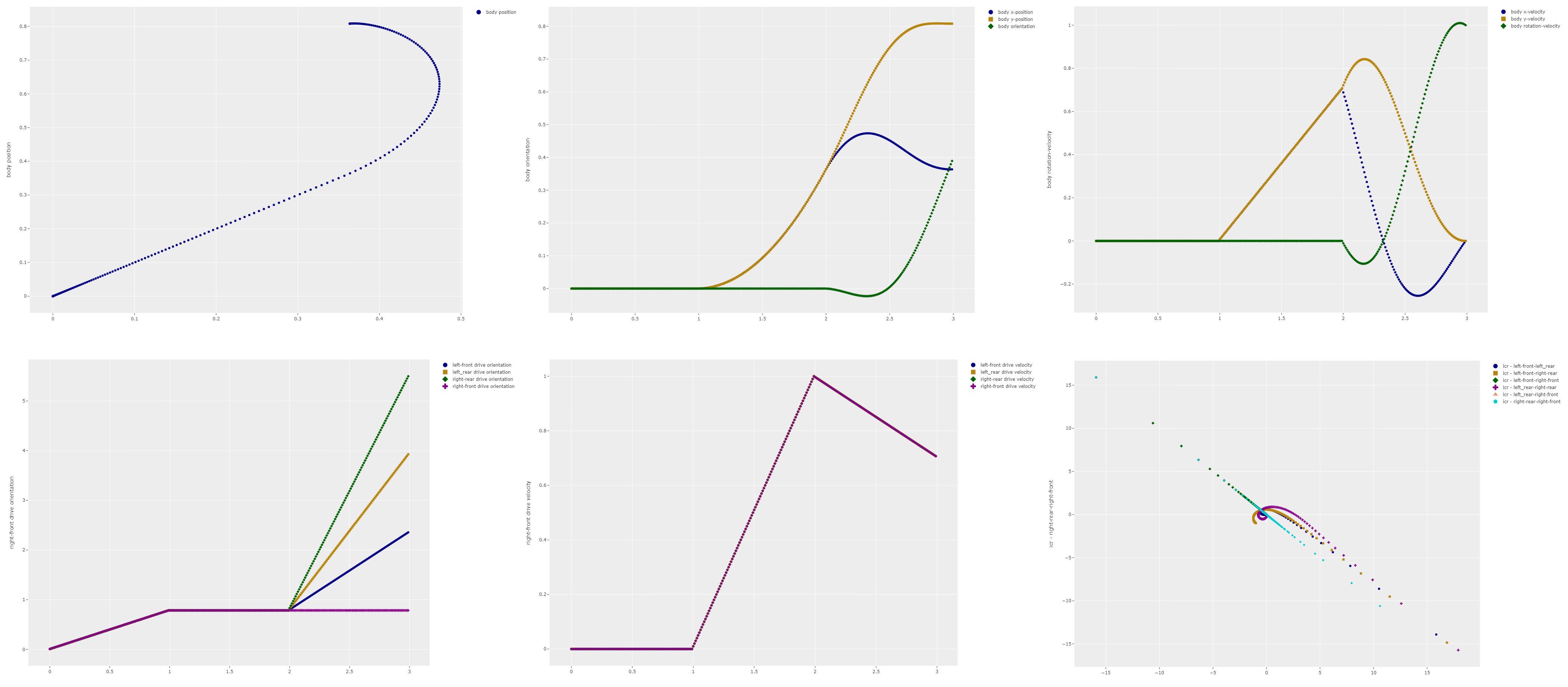
The benefit of controlling the robot by directly controlling the drive modules is that the control algorithm is very simple and all movement patterns are possible. For instance it is possible to make all the wheels change steering angle without moving the robot body, something which is not possible with indirect control methods.
However there are also a number of drawbacks. The main one is that for a swerve drive to be efficient the motions of the different drive modules need to be synchronized. That means that all the drive modules needs to be controlled so that none of the wheels slip along the surface. For simple linear or rotational movements of the robot body this is easy to achieve but for complicated movements this is much more difficult. An example is shown in image above which describes the behaviour of the robot as it moves linearly at a 45 degree angle and then transitions to an in-place rotation around the robot centre axis. The bottom right graph shows the instantaneous centre of rotation calculated for different combinations of two wheels. In a synchronised motion all wheels should point to the same instantaneous centre of rotation at any given moment. If the ICR's for the different wheel pairs are in different locations then one or more of the wheels is out of sync and likely slipping along the ground. The graph clearly shows that in this case the drive modules are not synchronized thus causing wheel slip.
One way to improve the synchronization between the drive modules is apply the movement control at an indirect level, for instance on the robot body, and then to work out from there what the drive modules should be doing at any that given point in time along the transition profile.
As with the previous approach I will use a linear profile to determine the transitions between different body states. Then the transition for the body velocities (x-velocity, y-velocity, and rotational velocity) can be determined from the start state to the end state. Once it is known what the body motion looks like I can calculate the states for the drive modules from the body state for all given states in the transition profile.
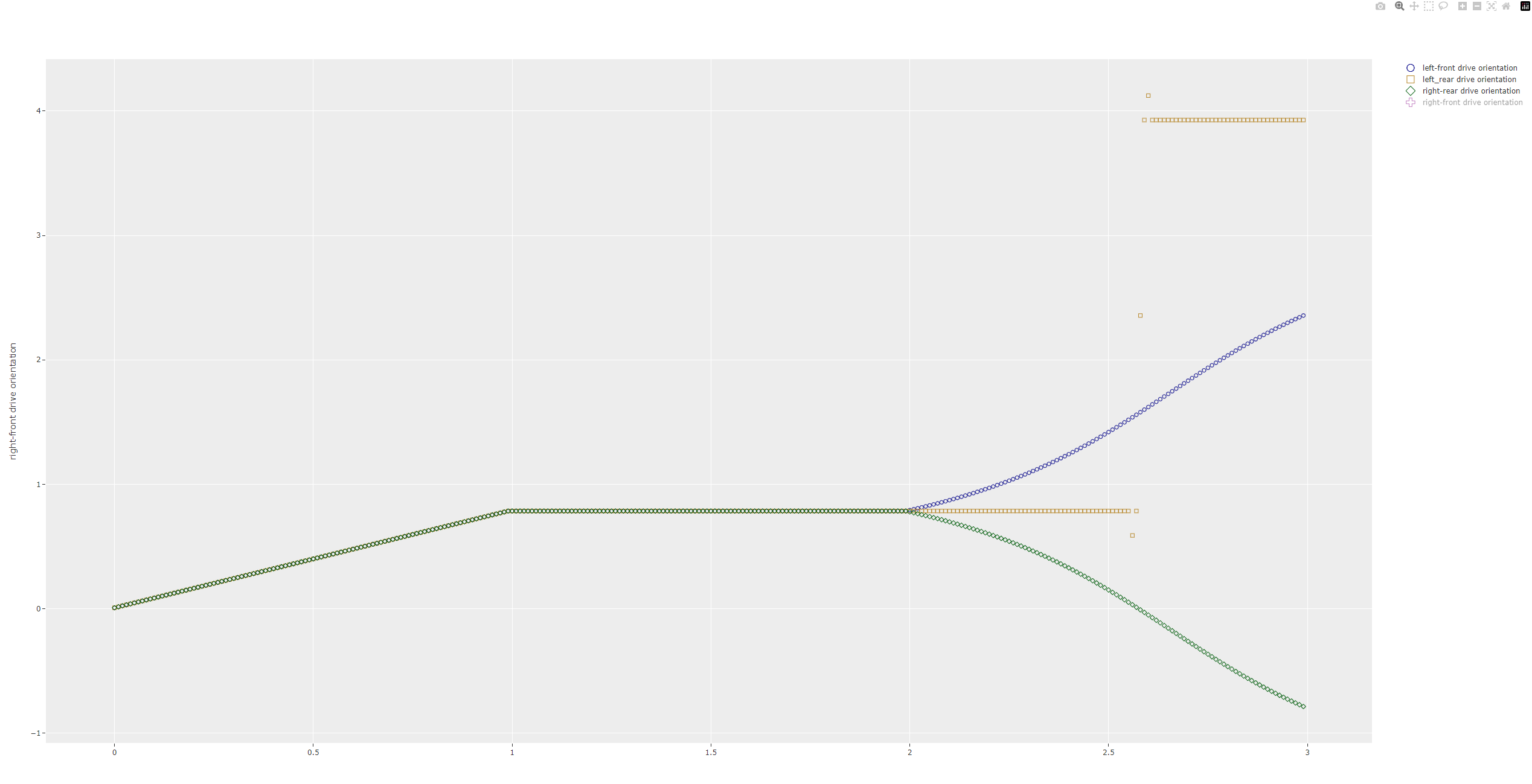
One issue with this approach is that every body state can be achieved by two different module states, one with the wheel moving ‘forward’ and one with the wheel moving 'backward'. Initially the simulation was hard-coded to always select the ‘forward’ moving state. However this leads to situations where the steering angle is flipped 180 degrees very rapidly. This is shown in the figure where the yellow line switches from 45 degrees (or 0.78 radians) to 225 degrees (or 3.9 radians) in two time steps, or 0.02 seconds. In real life this change in steering angle would likely not be possible because the steering angle motor would not be capable of delivering the enormous velocities and accelerations necessary to achieve this change.
To resolve this issue the simulation calculated the difference in rotation and velocity between the current point in time and the previous point in time along the transition profile, for both the forward and backward motions. Then general rule is to pick the smallest change in both rotation and velocity of the drive module. If that isn't possible then we pick the one with the smallest rotation difference for no real reason other than we have to pick something. In future work a more thorough algorithm will be implemented.
With all that code in place the simulation delivers a much smoother result for the transition from a 45 degree linear motion into a in-place rotation. The ICR path for all the wheel pairs is following a single path indicating that all the drive modules are all synchronised during the movement transition.
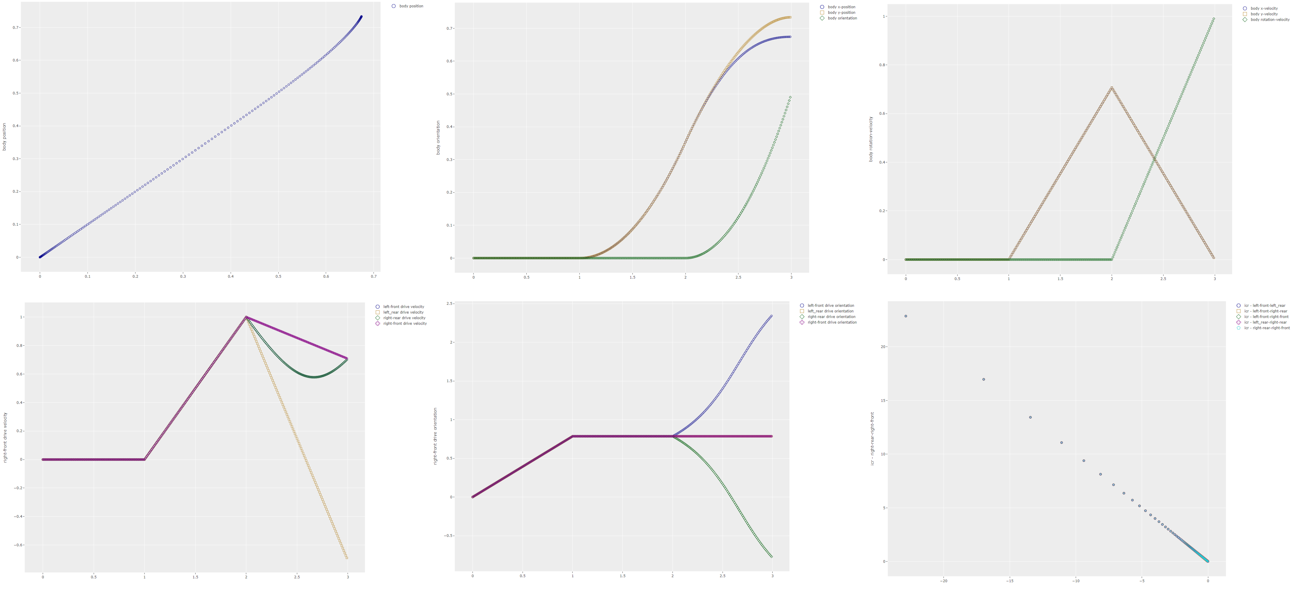
The body oriented control approach ensures synchronisation of the drive modules while allowing nearly all the different motions a swerve drive can make. The only motions not possible are those that involve drive module steering angle changes only.
The next improvement will be to replace the linear interpolation between the start state and the desired end state with a control approach that will provide smooth transitions for velocity and accelerations. This will make the motions of the robot less jerky and thus less likely to damage parts while also providing a smoother ride for the payload.
Edits
- July 4th 2023: Changed the term
control trajectorytocontrol profilebecause the termtrajectoryis generally reserved for path planning situations. - July 4th 2023: Changed the term
ICR trajectorytoICR pathbecause the the ICR does not follow a trajectory, it follows a path.