
Swerve drive - Motion profiles
In the last few posts I have described the simulations I did of a robot with a swerve drive. In other words a robot with four wheels each of which is independently driven and steered. I did simulations for the case where we specified movement commands directly for the drive modules and one for the case where we specified movement commands for the robot body which were then translated in the appropriate movements for the drive modules. One of the things you can see in both simulations is that the motions is quite ‘jerky’, i.e. with sudden changes of velocity or acceleration. In real life this kind of change would be noticed by humans as shocks which are uncomfortable and can potentially cause injury. For the equipment, i.e. the robot parts, a jerky motion adds load which can cause failures. So for both humans and equipment it is sensible to keep the 'jerkiness' as low as possible.
In order to achieve this we first need to understand what jerk actually is. Once we understand it
we can figure out ways to control it. Jerk is defined as the change of acceleration
with time, i.e the first time derivative of acceleration. So jerk vector as a function of time,
Where
t is time.\frac{{d}}{{dt}} ,\frac{{d}}{{dt^{2}}} ,\frac{{d}}{{dt^{3}}} are the first, second and third time derivatives.\vec{{a}} is the acceleration vector.\vec{{v}} is the velocity vector.\vec{{r}} is the position vector.
From these equations we can for instance deduce that a linearly increasing acceleration is caused by a constant jerk value. And a constant jerk value leads to a quadratic behaviour in the velocity. A more interesting deduction is that an acceleration that changes from a linear increase to a constant value means that there must be a discontinuous change in jerk. After all a linear increasing acceleration is caused by a constant positive jerk, and a constant acceleration is achieved by a zero jerk. Where these two acceleration profiles meet there must be a jump in jerk.
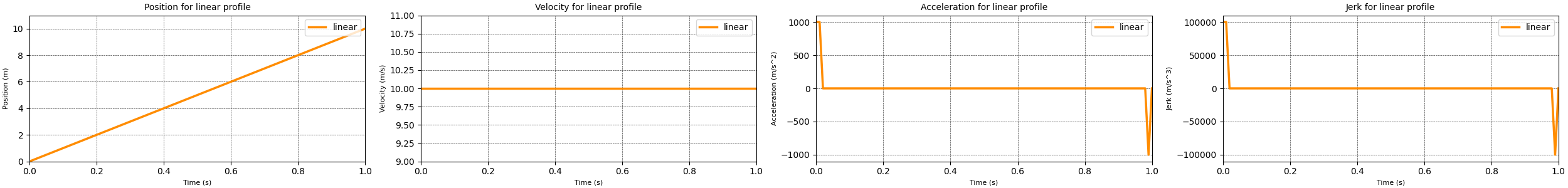
With that you can probably imagine what happens if the velocity has a change from a linearly increasing value to a constant value. The acceleration drops from a positive constant value to zero. And the jerk value displays spikes when the acceleration changes. For the linear motion profile this behaviour is amplified as shown in the plot below. The change in position requires a constant value for velocity which requires significant acceleration and jerk spikes at the start and end of the motion profile.
So in order to move a robot, or robot part, from one location to another in a way that the jerk values stay manageable we need to control the velocity and acceleration across time. This is normally done using a motion profile which describes how the velocity and acceleration change over time in order to arrive at the new state at the desired point in time. Two of the most well known motion profiles are the trapezoidal profile and the s-curve profile.
The trapezoidal motion profile
The trapezoidal motion profile consist of three distinct phases. During the first phase a constant positive acceleration is applied. This leads to a linearly increasing velocity until the maximum velocity is achieved. During the second phase no acceleration is applied, keeping the velocity constant. Finally in the third phase a constant negative acceleration is applied, leading to a decreasing velocity until the velocity becomes zero.
The equations for the different phases are as follows
The acceleration, velocity and position in each phase of the trapezoidal motion profile can be described with the standard equations of motion.
Where
t is the amount of time spend in the current phase.n is the current phase
For my calculations I assumed that the acceleration phase and the deceleration phase take the same amount of time, thus they have the same acceleration magnitude but different signs. With this the differences for each phase are:
a(t) = a_{{max}} a(t) = 0 a(t) = -a_{{max}}
My implementation
To simplify my implementation of the trapezoidal motion profile I assumed that the different stages of the profile all take the same amount of time, i.e. one third of the total time. In real life this may not be true because the amounts of time spend in the different stages depend on the maximum reachable acceleration and velocity as well as the minimum and maximum time in which the profile needs to be achieved. Making this assumption simplifies the initial implementation. At a later stage I will come back and implement more realistic profile behaviour.
Additionally my motion profile code assumes that the motion profile is stored for a relative timespan of 1 unit. If I want a different timespan I can just multiply by the desired timespan to get the final result. For this case we can now determine what the maximum velocity is that we need in order to travel the desired distance.
Where
t_{{accelerate}} is the total time during which there is a positive acceleration, which is one third of the total time.t_{{constant}} is the time during which there is a constant velocity, which is also one third of the total time.t_{{decelerate}} is the time during which there is a negative acceleration, which again is one third of the total time.
Simplifying leads to
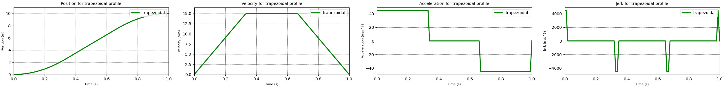
Using this maximum velocity and the equations for the different phases I implemented a trapezoidal motion profile. The results from running this motion profile are displayed in the plots above. These plots show that the trapezoidal has no large spikes in the acceleration profile when compared to the linear motion profile. additionally the jerk spikes for the trapezoidal motion profile are significantly smaller than the ones generated by the linear motion profile. So we can conclude that the trapezoidal motion profile is a better motion profile than the linear profile. However there are still spikes in the jerk values that would be detrimental for both humans and machinery. So it would be worth finding a better motion profile. That motion profile is the s-curve motion profile discussed in the next section.
The s-curve motion profile
Where the trapezoidal motion profile consisted of three different phases, the s-curve motion profile has seven distinct phases:
- The ramp up phase where a constant positive jerk is applied. Which leads to a linearly increasing acceleration and a velocity ramping up from zero following a second order curve.
- The constant acceleration phase where the jerk is zero. In this phase the velocity is increasing linearly.
- The first ramp down phase where a constant negative jerk is applied. This leads to a linearly decreasing acceleration until zero acceleration is achieved. The velocity is still increasing, following a slowing second order curve to a constant velocity value.
- The constant velocity phase where the jerk and acceleration are both zero.
- The first part of the deceleration phase where a constant negative jerk is applied. Again this leads to a linearly decreasing acceleration, and a velocity decreasing following a second order curve.
- In this phase the acceleration is kept constant and the velocity decreases linearly.
- The final phase where a constant positive jerk is applied with the goal to linearly increase the acceleration until zero acceleration is reached. The velocity will keep decreasing following a second order curve, until it too reaches zero.
As with the trapezoidal motion profile, the acceleration, velocity and position in each phase of the s-curve motion profile can be described with the standard equations of motion. The difference is that the acceleration is a linear function, which introduces a jerk value to the equations.
Where
t is the amount of time spend in the current phase.n is the current phase
As with the trapezoidal motion profile I assumed that the acceleration and deceleration phases span the same amount of time. Again this means the acceleration and deceleration have magnitude but different signs. The differences for each phase are:
j(t) = j_{{max}} j(t) = 0 j(t) = -j_{{max}} j(t) = 0 ,a(t) = 0 j(t) = -j_{{max}} j(t) = 0 j(t) = j_{{max}}
My implementation
To simplify my implementation of the s-curve motion profile I assumed that all stages, except stage 4, all take the same amount of time, i.e. one eight of the total time. I assumed that stage 4 would take one quarter of the time. Like with the trapezoidal profile making this assumption simplifies the initial implementation. At a later stage I will come back and implement more realistic profile behaviour.
Additionally my motion profile code assumes that the motion profile is stored for a relative timespan of 1 unit. If I want a different timespan I can just multiply by the desired timespan to get the final result. For this case we can now determine what the maximum velocity is that we need in order to travel the desired distance.
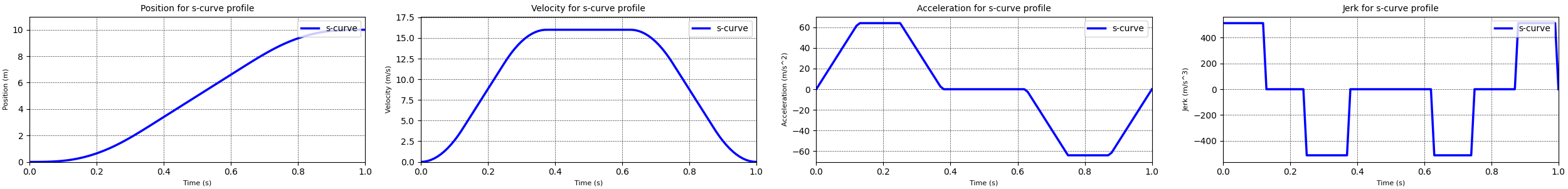
Using the equations above I implemented a s-curve motion profile. The results from running this motion profile are displayed in the plots above. These plots show that the s-curve removes the spikes in the jerk profile when compared to the trapezoidal motion profile. This indicates that the s-curve motion profile achieves the goal we previously set, to minimize the jerky motion.
For some applications it is important to provide even smoother motions. In this case the motion profiles may need to take into account the values of the fourth, fifth or even sixth order time derivatives of position, snap, crackle and pop. At the moment I have not implemented these higher order motion profiles.
Use in the swerve simulation
Having these motion profiles is great, however by themselves they are of little use. So I added them to my swerve drive simulation to see what the differences were between the different motion profiles.
Before we look at the new results it is worth looking at the simulations using the linear motion profile. I made one for module control and one for body control. In these simulations you can see that with the linear motion profile the jerk spikes are quite large, especially in the case of the module control simulation. The body control approach performs a little better with respect to the maximum levels of jerk, however the values are still far too high.
The simulations for module control and body control using the trapezoidal profile show a significant decrease in the maximum value of the acceleration and jerk values, in some cases by a factor 15. As expected from the previous discussion there are still some spikes, especially for the steering angles. The changes for the module control case are more drastic than for the body control case, probably due to the fact that the values were very high for the combination of the module control with a linear motion profile. Interestingly the acceleration and jerk maximum values are lower for the module control approach than they are for the body control approach. This is most likely due to the fact that in order to keep the drive modules synchronised relatively high steering velocities are required. For instance, the module control approach using the trapezoidal motion profile sees a maximum steering velocity of about 1.8 radians per second. Compare this to the the body control approach with the trapezoidal motion profile which sees a maximum steering velocity of about 3.8 radians per second.
When we look at the simulations using the s-curve motion profile we can see that the maximum acceleration and jerk values actually increase when compared to the trapezoidal motion profile, except for the values of the steering angle jerk when using the module control approach. It seems likely that these increases are due to the fact that the motion is executed over the same time span, but some of the time is used for a more smooth acceleration and deceleration. This means that there is less time available to travel the desired ‘distance’ which then requires higher maximum velocities and maximum accelerations. The s-curve motion profile does smooth out the movement profiles which would lead to a much smoother ride.
What is next
So now that we have a swerve drive simulation that can use both module based control and body based control as well as have different motion profiles, what is next? There are a few improvements that can be made to the simulation code to further made to the simulation and a path of progression.
The first improvement lies in the fact that none of the motion profiles, linear, trapezoidal and s-curve, are aware of motor limits. This means that they will happily command velocity, acceleration and jerk values that a real life motor would not be able to deliver. In order to make the simulation better I would need to add some kind of limits on the maximum reachable values. This would be especially interesting when using body oriented control. Because the high velocities and accelerations are needed to keep the drive modules synchronised. If one of the drive modules is not able to reach the desired velocity or acceleration then the other modules will have to slow down before they reach their limits. To control the drive modules in such a way that all of the modules stay within their motor limits while also keeping them synchronised requires some fancy math. At the moment I'm going through a number of published papers to see what different algorithms are out there.
The second improvement that is on my mind is to implement some form of path tracking, i.e. the ability to follow a given path. This would give the simulation the ability to better show the behaviour of a real life robot. In most cases when a robot is navigating an area the path planning code will constantly be sending movement instructions to ensure that the robot follows the originally planned path. This means that motion profiles need to be updated constantly, which will be a challenge for the simulation code. Additionally having path tracking in the simulation would allow me to experiment with different algorithms for path tracking and trajectory tracking, i.e. the ability to follow a path and prescribe the velocity at every point on the path. And theoretically with a swerve drive it should even be possible for the robot to follow a trajectory while controlling the orientation of the robot body.
Finally the path of progression is to take the controller code that I have written for this simulation and use it with my ROS2 based swerve robot.