
Swerve drive - Kinematics simulation
As mentioned I am designing and building four wheel steering mobile robot for use in outdoor environments and rough terrain. In that post I mused that both the mechanical design and the software would be the most complicated parts of the drive system and thus the parts I should focus on first. At the moment I don't have good access to a workshop where I can experiment with the mechanical design so for now I'm focussing on the creation of the control software. Once I have the controller software working I can then use Gazebo to test the robot virtually to ensure that the code will work in the actual robot.
Unlike a differential drive a four wheel swerve drive has more degrees of freedom than needed, eight degrees of freedom (steering angle and wheel velocity for each drive module) for the control versus three spatial degrees of freedom (forward, sideways and rotate). This means that a swerve drive is an over-determined system, requiring the control system to carefully control the wheel velocities and angles so that they agree with each other, otherwise the wheels slip or drag.
While doing some research I found many different scientific papers describing algorithms for determining the forward and inverse kinematics of a four wheel steering system. There are however very few software libraries which implement the different control algorithms.
Most papers and libraries focus on the simpler case of an indoor robot that moves along a flat horizontal surface. In this case relatively simple kinematics approaches can be used. Unfortunately these algorithms fail when used in 3d uneven terrain. A different approach is required for that case. At the moment I too will be focussed on algorithms for driving on flat surfaces. At least until I have correctly working control code.
After reading a number of papers and looking at some of the available code I have come to the conclusion that I don't understand what is required for a successful swerve algorithm. There are many variables that influence the behaviour making it hard to visualize what goes on as the robot is moving around. So I wrote some code to simulate what is going on (roughly) in a swerve drive while it is moving and steering. I'm going to use this code to answer a number of questions I have about the different control algorithms.
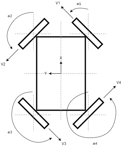
For instance algorithms often calculate the desired end state and then set the wheel position and velocity to those required for that desired state. The question is does this algorithm automatically ensure that the intermediate states are synchronised, and if not does that matter? An example of this would be a robot moving linearly at 45 degrees and transitioning to an in-place rotation, as pictured below. During the transition all drive modules should be synchronised so that the center of rotation for the robot matches with the state of the drive modules.
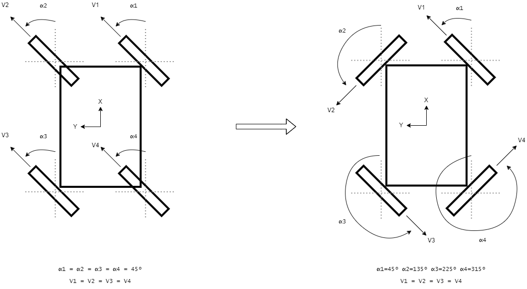
Another example is that many of the code libraries add an optimization that reverses the wheel direction in favour of reducing the steering angle. For instance instead of changing the steering angle from 0 degrees to 225 degrees with a wheel velocity of 1.0 rad/s, change the angle to 45 degrees and reverse the wheel velocity to -1.0 rad/s. Again there are a number of questions about this optimization. For instance making a smaller steering angle change reduces the energy used, however stopping and reversing the wheel motion also takes energy, so what are the benefits of this optimization, if any? And how do the algorithms keep the wheel motions synchronised when performing the reversing optimization?
The following graphs show an example of the simulation output. The motion being simulated is that of a robot transiting from moving at a 45 degree straight path to an in-place rotation. The graphs display the status of the robot body, position and velocity and the status of the different drive modules, the angular orientation and the wheel velocity. The last graph depicts the location of the Instantaneous Centre of Rotation (ICR) for different combinations of drive modules. The ICR is the point in space around which the robot turns. If the control algorithm is correct then the ICR points for different drive module combinations all fall in the same location though out the entire movement pattern.
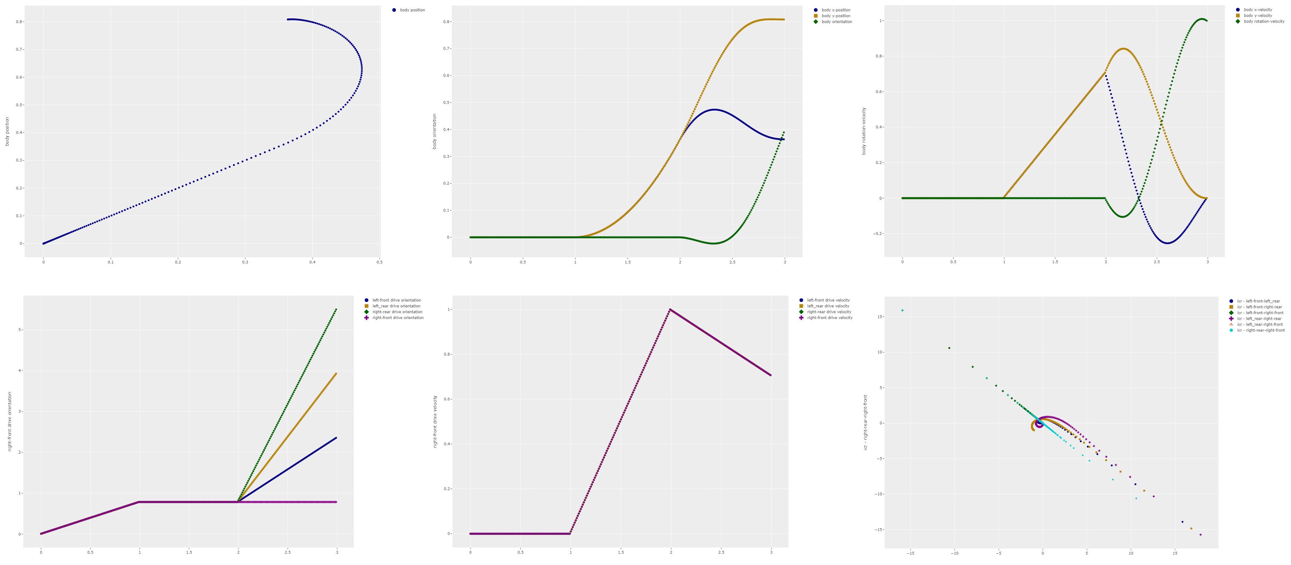
Looking at these graphs a couple of observations can be made. The first observation is that the ICR paths for the different module combinations don't match each other. This means that the drive modules are not synchronised and one or more wheels will be experiencing wheel slip. The second observation is that the linear control algorithm causes sharp changes in velocities leading to extremely high acceleration demands. It seems unlikely that the motors and the structure would be able to cope with these demands.
From this relatively simple simulation we can see that there are a number of behaviours that the control system needs to cope with:
- The state of the drive modules actively needs to be kept in sync at all times, including during transitions from one movement state to another. This indicates that dynamic control is required and thus poses questions about the update frequency for drive module sensors and control commands.
- The capabilities and behaviour of the motors needs to be taken into account in order to prevent impossible movement commands and also to ensure that the drive modules remain synchronised during movement commands that require fast state changes from the motors, e.g. to deal with motor deadband or fast accelerations.
- The structural and kinematic limitations need to be considered when giving and processing movement commands.
- Linear control behaviour is not ideal as it causes large acceleration demands so a better approach is necessary.
Now that I have some working simulation code what are the next steps? The first stage is to simulate some more simple movement trajectories to validate the simulation code. Once I have confidence that the code actually simulates real world behaviour I can implement different control algorithms. These algorithms can then be compared to see which algorithm behaves the best. Currently I'm thinking to implement
- A control algorithm that uses a known movement profile for the robot base. It can then calculate the desired drive module state across time to match the robot base movement. The movement profile could be linear, polynomial or any other sensible profile.
- A controller that optimizes module turn time by having it turn the shortest amount and reversing the wheel velocity if required.
- A low jerk controller that ensures smooth movement of the robot body and drive modules.
In future posts I will provide more details about the different controller and model algorithms.