
Swerve drive - Movement animations
In my last two posts I talked about different control methods for a swerve drive robot. One method controls the movement of drive modules directly. The other method controls the movement of the body and derives the desired state for the drive modules from that.
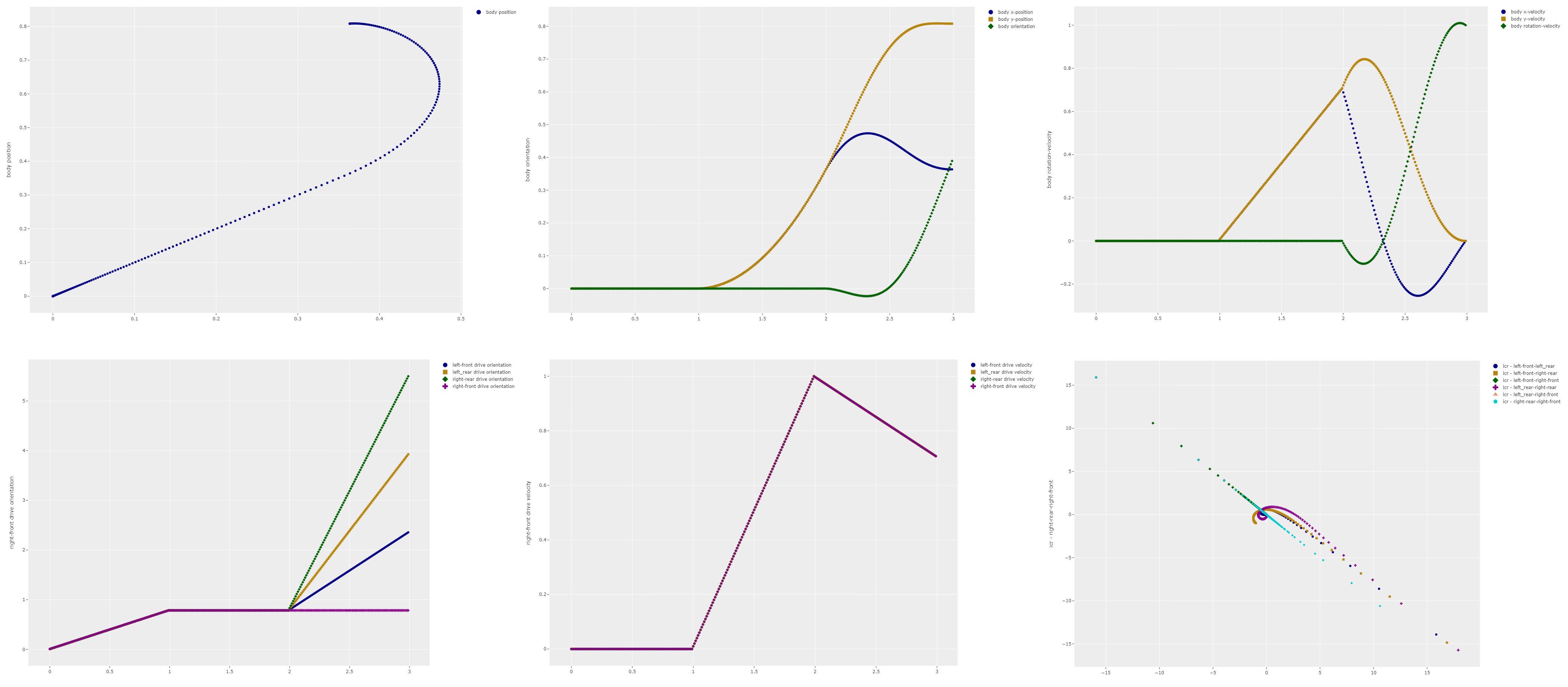
To see the difference between these control methods my simulation code created all kinds of interesting plots like the ones above. However I was still having trouble visualizing what was actually happening, especially in the case of the movement of the Instantaneous Centre of Rotation (ICR), i.e. the rotation point for the robot at a given point in time. The lower left graph shows the paths the ICR for different combinations of drive modules. While it looks pretty it does not make a lot of sense to me.
So to address that issue I updated the simulation code to produce some animations that display the position of the robot and the wheels as well as a number of plots for the state of the robot body and the drive modules. To create the animations I used the FuncAnimation class that is available in matplotlib. The animations can then either be turned into an HTML page with animation controls using the HTMLWriter, or into MP4 video files using the FFMpegWriter. In order to get reasonable performance when using the animation functions in matplotlib it is important to update the plots instead of drawing new ones. This can be done using the set_data function, for instance for updating the position of the robot body. It is good to keep in mind that even with this performance improvement the creation of the animations isn't very fast for our robot simulation because a large number of image frames need to be made. For the 6 second movement in the animation anywhere between 150 and 600 frames need to be created.
The animation above shows how the robot behaves when using the direct module controller. As you can see in the video different pairs of wheels have different rotation points, signified by the red dots. As the movement progresses these rotation points have quite a large range of motion. This indicates that the wheels are not synchronized and most likely some of the wheels are slipping.
I created another animation for the same situation but with the body oriented controller. In this case the rotation points are all in a single location leading me to conclude that all the wheels are synchronized and little to no wheel slip is occurring.
One other interesting thing you can see in the video is that the acceleration and jerk values change very abruptly. In real life this would lead to significant loads on the robot and its drive system. In the simulation this behaviour is due to the fact that linear profile that is being used to transition from one state to another. As mentioned before the next improvement will be to replace this linear interpolation with a control approach that will provide smooth transitions for velocity and accelerations.
Edits
- July 6th 2023: Added a section discussing the use of the matplotlib animation functions.