
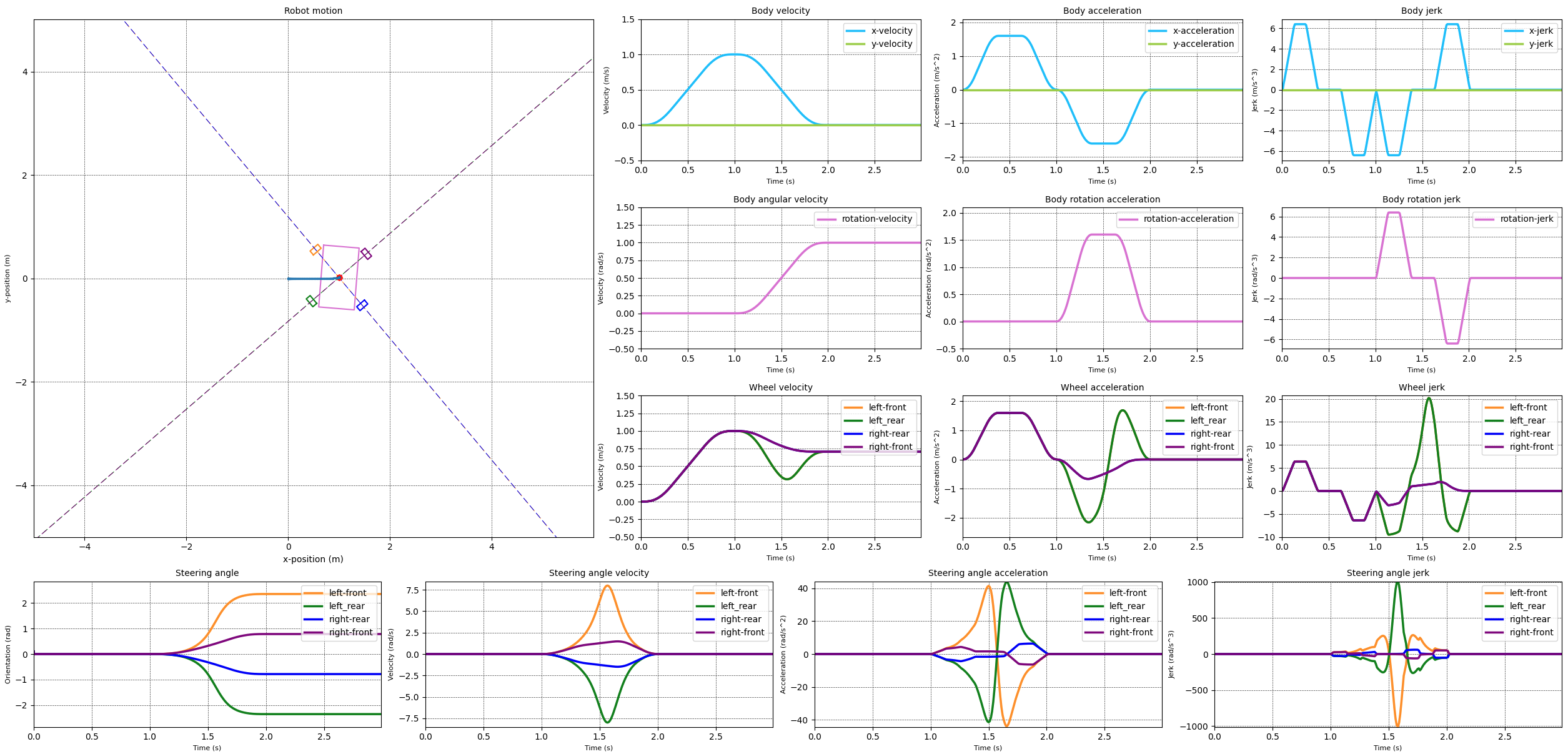
The swerve controller I have implemented so far assumes that the robot is able to follow all the movement commands it has been given. This can lead to extreme velocity and acceleration for the drive and steering motors. The image below shows the result of a simulation where the robot is commanded to move in a straight line followed by a rotate in-place. The simulation used a s-curve motion profile to generate a smooth body movement between different states. The graphs show that the drive velocity and acceleration are smooth and don't reach very high values. It is thus expected that these are well within the capabilities of the drive motors. The steering velocity and acceleration show significant peaks which are likely to tax the steering motors.
In order to ensure that the motors are able to follow the movement commands while keeping the motions of the different drive modules synchronised, we need to take into account the capabilities of the motors.
Now there are many different motor characteristics that we could take into account. For instance:
- The maximum velocity the motor can achieve. This obviously limits how fast the drive module can steer or rotate the wheels.
- The maximum acceleration the motor can achieve. This limits how fast the drive module can change the drive or steering velocity and thus how quickly it can respond to command changes.
- The maximum jerk the motor can achieve. This limits how quickly the motor can achieve the desired acceleration.
- The existence of any motor deadband. This is the region around zero rotation speed where the motor doesn't have enough torque to overcome the static friction of the motor and attached systems. Once enough torque is applied the motor will start running at the rotation speed that it would normally have for that amount of torque. This means that there is a minimum rotation speed that the motor can achieve.
- The behaviour of the motor under load. For instance the motor may not be able to reach the desired rotation speed under load.
- The motor settling time, which is the time it takes the motor to reach the commanded speed.
- The behaviour of the motor when running ‘forwards’ versus when running 'backwards'. For instance the motor may have a different maximum velocity in the ‘forward’ direction than it does in the 'backwards' direction.
At the moment I will only be looking at the maximum motor velocities and the accelerations. These two have a direct effect on the synchronisation between the drive modules. The other characteristics will be dealt at a later stage as they require more information and thought.
In order to limit the steering and drive velocities I've implemented the following process
- Determine the body movement profile that allows the body to achieve the desired movement state in a smooth manner using s-curve motion profiles.
- Divide the body movement profiles into N+1 points, dividing the profile into N sections of equal time. For each of these points calculate the velocity and steering angle for the drive modules. These velocities and steering angles then form the motion profiles for each of the drive modules.
- For each point in time check the steering velocity for each module. Record the maximum velocity of all the profiles. If the maximum velocity is larger than what the motor can deliver then increase or decrease the current timestep in order to limit the steering velocity to the maximum velocity of the motor. Changing the duration of the timestep will change the steering velocities of all the modules. Thus we limit the steering velocities while maintaining synchronisation between the modules.
- Repeat the previous step for the drive velocities.
The following video shows the result of the simulation using the new velocity limiter code. The video shows the robot moving in a straight line and then rotating in place. When the rotation starts the steering velocity for the different drive modules increases. As the steering velocity reaches 2 rad/s for the left front and left rear modules the limiter kicks in and maintains that steering velocity. In response the steering velocities of the other wheels reduces in order to keep the drive modules synchronised. The wheel velocities are slightly altered.
With the steering and wheel velocities limited in a reasonable way I attempted to do the same for the steering acceleration. The results of this can be seen in the next images. The first image limits the steering acceleration to 15 rad/s^2. The second image limits the steering acceleration to 10 rad/s^2.
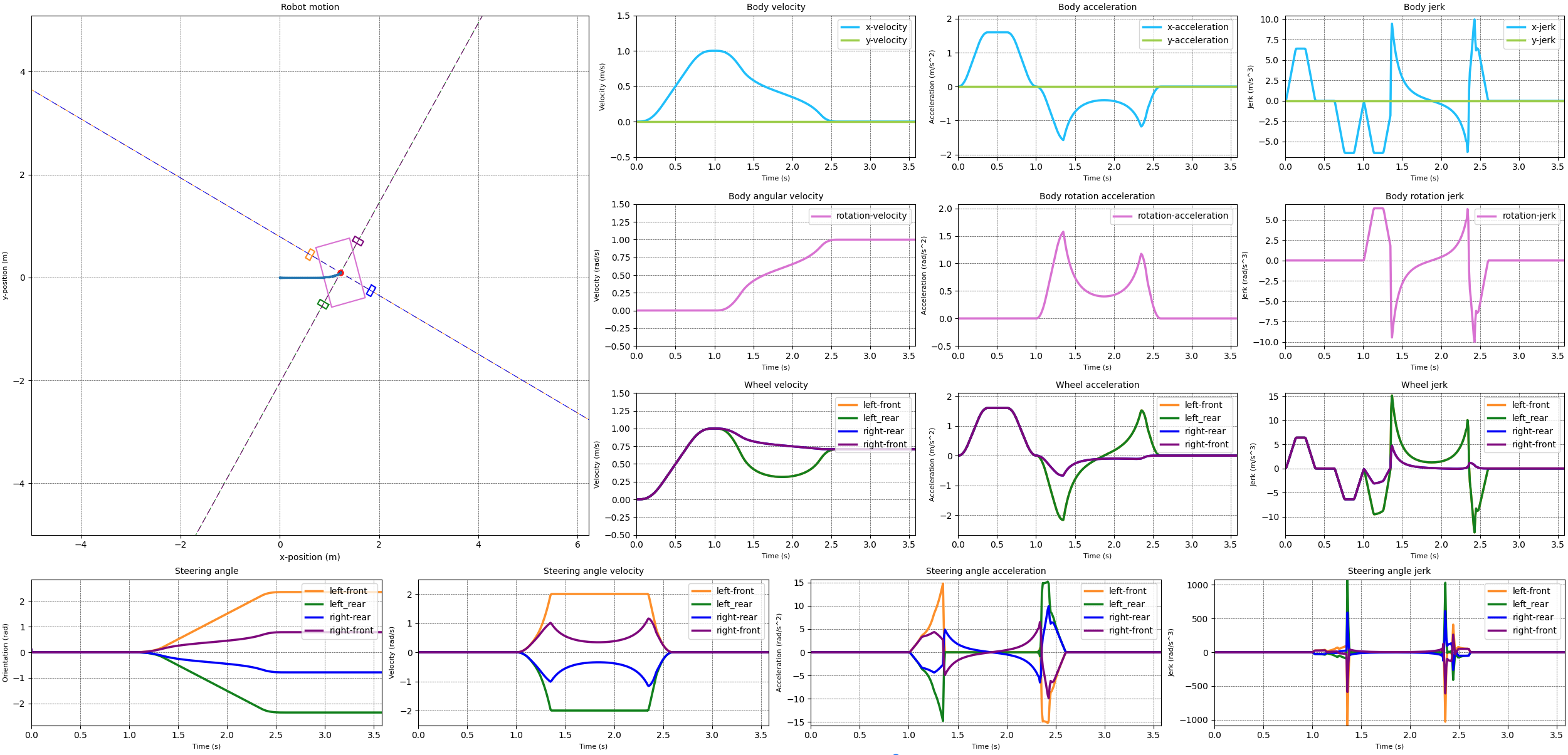
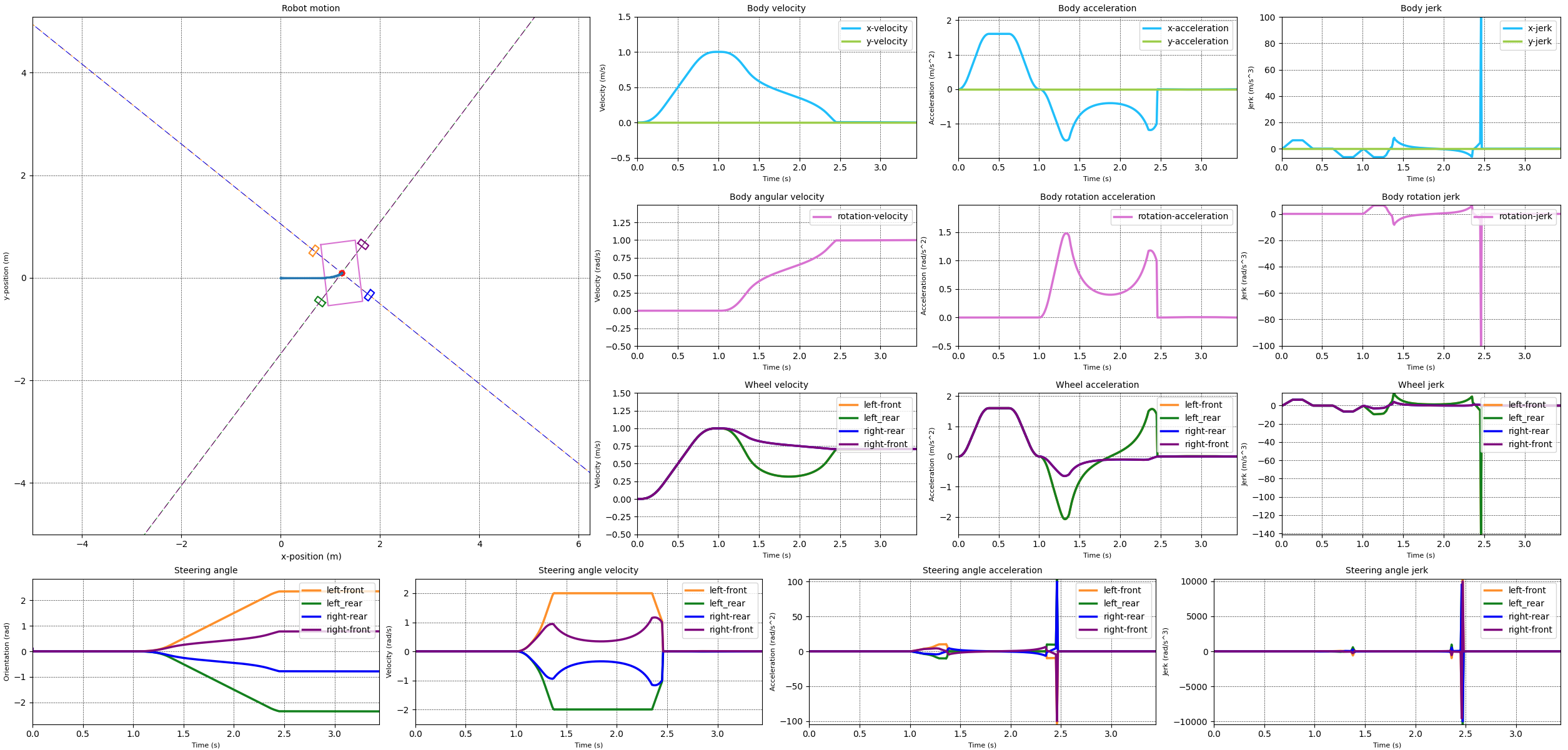
When comparing the two simulation results it becomes clear that something happens if we limit the steering acceleration to 10 rad/s^2. The velocities over all for both cases looks reasonable, except for the 10 rad/s^2 case where the steering velocity snaps to zero at the end of the transition from the straight line to the rotation. This is reflected in a momentary acceleration of over 100 rad/s^2.
The acceleration is calculated based on the difference between the velocity at the current timestep and the velocity at the previous timestep. Additionally the algorithm has to ensure that the steering angle change between the previous and current timestep is controlled so that synchronisation of the drive modules is maintained. Generally to limit the velocity the duration of the timestep is increased. However for the acceleration, especially when decelerating from a positive velocity, there is a limit to how much the timestep can be increased. A larger time step increase decreases the velocity. This then increases the deceleration needed. So this means that you get very large timesteps, or very small timesteps. The current algorithm favours small timesteps.
In either case the problem occurs when slowing down. At the end of the deceleration profile the desired position is achieved, but the velocity and acceleration are not zero. This is not realistic or physically possible. This behaviour is possibly due to the fact that the timesteps are individually calculated. This means that the algorithm doesn't know what the desired end states are and so those are not taken into account.
Additionally if we look at this approach from a higher level we can see that there are two potential areas where improvements can be made in the control model. The first area is related to the fact that the steering velocity and acceleration are computed values, i.e. they are derived from the change in the steering position. This means that there is no direct control over the steering velocity and acceleration. A better algorithm would include these values directly and be able to apply boundary conditions on these values. This could be achieved by extending the current kinematic model with the body accelerations and jerks. The second area is related tot the fact that the module states are derived from the body state. This is necessary to keep the modules synchronised with the body. However this means that the module states are not directly controlled. Which means that it is more difficult to include the module limitations in the control model.
These issues will only become more pronounced if we want to start limiting the maximum jerk values for the steering and drive directions. Limiting the maximum jerk is required to prevent excessive forces on the drive module components.
One possible solution to these issues is to switch to a dynamic model for the control of the robot, i.e. one that is based on the forces and accelerations observed by the robot as it moves. The current model is a kinematic model, i.e. based on the positions and velocities of the different components. Using a dynamic model would allow for the inclusion of the body accelerations and jerks. Additionally the dynamic model would allow for the inclusion of the behaviour of the steering modules more directly and thus lead to a more accurate control model. Finally a dynamic model would also allow for the inclusion of skid and slip conditions as well as three dimensional movement on uneven terrain. The drawback of a dynamic model is that it is more complex and thus requires more effort during implementation and at run time.
At the moment I have not made any decisions on how to progress the swerve controller. It seems logical to implement a dynamic model, however which model should be used and how to implement it requires a bit more research. For the time being I'm planning my next step to be to design and build a single drive module in real life.
The goals for the development of my swerve drive robot were to develop an off-road capable robot that can navigate autonomously between different locations to execute tasks either by itself or in cooperation with other robots. So far I have implemented the first version of the steering and drive controller, added motion profiles for smoother changes in velocity and acceleration, and I have created the URDF files that allow me to simulate the robot in Gazebo. The next part is to add the ability to navigate the robot, autonomously, to a goal location.
So how does the navigation in general work? The first step is to figure out where the robot is, or at least what is around the robot. Using the robot sensors, e.g. a lidar, we can see what the direct environment looks like, e.g. the robot is in a room of a building. If we have a map of the larger environment, e.g. the building, then using a location algorithm we can figure out where in the building we are. Assuming there are enough features in the room to make it obvious which room we are in. If we don't have a map of the environment then we can use a SLAM algorithm to create a map while the robot is moving. Having a map makes planning more reliable, because we can plan a path that takes into account the surroundings. However it is not strictly necessary, we can also plan a path without a map, but then it is possible that the planner will plan a path that is not possible to follow, e.g. because there is a wall in the way. Of course if there are dynamic obstacles, e.g. if a door is closed, then the map might not be accurate and we might still not be able to get to the goal.
Once the robot knows where it is and it has a goal location, it can plan a path from the current location to the goal location. This is generally done by a global planner or planner for short. There are many different algorithms for path planning each with their own advantages and disadvantages. Most planners only plan a path, consisting of a number of waypoints, from the current location to the goal location. More advanced planners can also provide velocity information along the path, turning the path into a trajectory for the robot to follow. Once a path, or trajectory, is created the robot can follow this path to reach the goal. For this a local planner or controller is used. The controller works to make the robot follow the path while making progress towards the goal and avoiding obstacles. Again there are a number of different algorithms, each with it own constraints.
Note that robot navigation is a very complex topic that is very actively being researched. A result of this is that there are many ways in which navigation can fail or not work as expected. For example some of the issues I have seen are:
- The planner is unable to find a path to the goal. This can happen when there is no actual way to get to the goal, e.g. the robot is in a room with a closed door with the goal outside the room. Or when the path would pass through a section that is too narrow for the robot to fit through.
- The controller is unable to follow path created by the planner, most likely because the path is not kinematically possible for the robot. For example the path might require the robot to turn in place when it is using an Ackerman steering system. Or the path requires the robot to pass through a narrow space that the controller deems to narrow.
- The robot gets stuck in a corner or hallway. It considers the hallway too narrow to fit through safely or has no way to perform the directional changes it wants to make. Sometimes this is caused by the robot being too wide. However most of the cases I have seen it in is caused by the planner configuration.
- The robot is slow to respond to movement commands, leading to ever larger commanded steering and velocities. This was mostly an issue with the DWB controller, the MPPI controller seems to be more responsive. However there is definitely an issue with the swerve controller code that I need to investigate.
- The VM I was running the simulation on wasn't quick enough to run the simulation close to real time. So at some point I need to switch to running on a desktop.
And these are only the ones I have seen. There are many more ways in which the navigation can fail. So it pays to stay up to date with the latest developments and to ensure that you have good ways to test and debug your robot and the navigation stack.
Now that we know roughly what is needed for successful navigation let's have a look at what is needed for the swerve drive robot. The first thing we need is a way to figure out where we are. Because I don't have a map of the environment I am using an online SLAM approach, which creates the map as the robot moves around the area. The slam_toolbox package makes this easy. The configuration for the robot is mostly the default configuration, except for the changes required to match the URDF model.
For the navigation I am using the Nav2 package. From that package I selected the SMAC lattice for the planner and the MPPI controller. These two were selected because they both support omnidirectional movement for non-circular, arbitrary shaped robots. The omnidirectional movement is required because the swerve drive robot can move in all directions and it would be a waste not to use that capability. The non-circular robot comes from the fact that the robot is rectangular and could pass through narrow passages in one orientation but not the other. Originally I tried the DWB controller and the navfn planner. Both are said to support omnidirectional movement. But when applied the DWB planner didn't really use the omnidirectional capabilities. Additionally it gets stuck for certain movements for unknown reasons. Once I changed to using the SMAC planner and the MPPI controller the robot was successfully able to navigate around the environment. Again the configuration is mostly the default configuration except that I have updated some of the values to match the robot's capabilities.
With all that set I got the robot to navigate to a goal. The video shows the robot starting the navigation from one room to another. As it moves at the 15 second mark it starts sideways translating while rotating to get around the corner in order to get through the door of the room. It continues its journey mostly traversing sideways, occasionally rotating into the direction it is moving. At the 52 second mark it reaches the goal location and rotates into the orientation it was commanded to end up in. Note that the planner inserted a turn, stop and back-up segment to get to the right orientation but the local planner opted to perform an in-place rotation at the end.
While there was a bit of tuning required to get the SLAM and navigation stacks to work, in the end it worked well. Obviously this is only one test case so once I have a dedicated PC to run the simulation I am going to do a lot more testing.
One of the things that is currently not implemented is limits on the steering and drive velocities. This means that currently the robot can move at any speed and turn at any rate. This is not realistic and will in the real world lead to the motors in the robot being overloaded. So the next step is to add the limits to the controller. The main issue with this is the need to keep the drive modules synchronised. So when one of the modules exceeds its velocity limits the other modules have to be slowed down as well so that we don't lose synchronisation between the modules. More on this in one of my next posts.
In a previous post I talked about simulating the SCUTTLE robot using ROS and Gazebo. I used Gazebo to simulate the SCUTTLE robot so that I could learn more about ROS without needing to involve a real robot with all the setup and complications that come with that. Additionally when I was designing the bump sensor for SCUTTLE using the simulation allowed me to reduce the feedback time compared to testing the design on a physical robot. This speeds up the design iteration process and allowed me to quickly and verify the design and the code. In the end you always need to do the final testing on a real robot, but by using simulation you can quickly iterate to a solution that will most likely work without major issues.
In order to progress my swerve drive robot I wanted to verify that the control algorithms that I had developed would work for an actual robot. Ideally before spending money on the hardware. So I decided to use Gazebo to run some simulations that would enable me to verify the control algorithm.
The first step in using Gazebo is to create a model of the robot and its surrounding environment. Gazebo natively uses the SDF format to define both the robot and the environment. However if you want ROS nodes to be able to understand the geometry definition of your robot you need to use the URDF format. This is important for instance if you want to make use of the tf2 library to transform between different coordinate frames then your ROS nodes will have to have the geometry of the robot available.
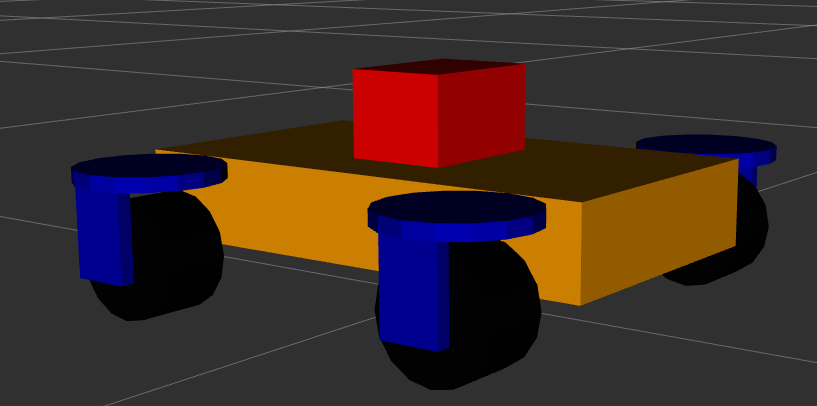
There are different ways to create an URDF model. One way is to draw the robot in a CAD program and then use a plugin to export the model to an URDF file. This is a relatively quick approach, it takes time to create the robot in the CAD program but then the export is very quick. The drawback of this method is that the resulting URDF file is not very clean which makes it harder to edit later on. Additionally the CAD software will use meshes for both the visual geometry and the collision geometry. As discussed below this can lead to issues with the collision detection. Another way is to create the URDF manually. This approach is slower than the CAD export approach, however it results in a much more minimal and clean URDF file. This makes editing the file at a later stage a lot easier. Additionally manually creating the URDF file give you a better understanding of the URDF format and how it works. In the end the model for my swerve drive robot is very simple, consisting of a body, four wheels, the steering and drive controllers and the sensors. So I decided to create the URDF file manually. The images below show the resulting model in RViz. The model consists of the robot body in orange, the four drive modules in blue and black, and the lidar unit in red.
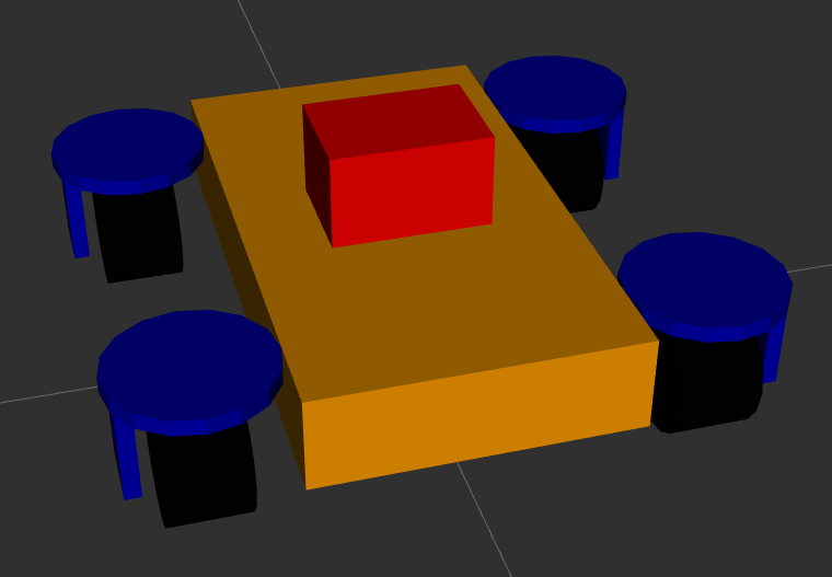
The URDF model describes the different parts of the robot relative to each other. The robot parts consist of the physical parts of the robot, the sensors and the actuators. The physical parts, e.g. the wheels or the body, are described using links. The links are connected to each other using joints. Joints allow the links to move relative to each other. Joints can be fixed, e.g. when two structural parts are statically connected to each other, or they can be movable. If a joint is movable then be one of:
- A revolute joint, which allows the two links to rotate relative to each other around a single axis.
- A continuous joint, which is similar to a revolute joint but allows the joint to rotate continuously without any limits.
- A prismatic joint, which allows the two links to move relative to each other along a single axis.
- A floating joint, which allows the two links to move relative to each other in 6 degrees of freedom.
- A planar joint, which allows the two links to move relative to each other in 3 degrees of freedom in a plane.
In the URDF file each link defines the visual geometry, the collision geometry and the inertial properties for that link. The visual and collision geometry can be defined either by a primitive (box, cylinder or sphere) or a triangle mesh. It is recommended to use simple primitives for the collision geometry since these make the collision calculations faster and more stable. If you use a triangle mesh for the collision geometry then you can get issues with the collision detection. This can lead to the robot moving around when it shouldn't. For instance when the wheel of the robot is modelled as a triangle mesh then the collision calculation between the wheel and the ground may not be numerically stable which leads to undesired movement of the robot. The current version of the SCUTTLE URDF has this problem as is shown in the video below. In a future post I'll describe how to fix this.
Using meshes for the visual geometry is fine as this geometry is only used for the visual representation of the robot. Note that the meshes should be relatively simple as well since Gazebo will have to render the meshes in real time which is expensive if the mesh consists of a large number of vertices and triangles.
I normally start by defining a link that represents the footprint
of the robot on the ground, called base_footprint. This link doesn't define any geometry, it is
only used to define the origin of the robot. When navigation is configured it will be referencing
this footprint link. The next link that is defined is the base_link. This link is generally defined
to be the ‘middle’ of the robot frame and it forms the parent for all the other robot parts.
The next step is to define the rest of the links and joints. For the swerve drive robot I have four drive modules, each consisting of a wheel and a steering motor. The wheel is connected to the steering motor using a continuous joint. The steering motor is connected to the base link using another continuous joint. Because the four modules are all the same I use the xacro format. This allows me to define a single module as a template and then use that template to create the four modules. The benefit of this is that it makes the URDF file easier to edit and a lot smaller and easier to read.
To add sensors you need to add two pieces of information, the information about the sensor body and, if you are using gazebo, the information about the sensors behaviour. The former consist of the visual and collision geometry of the sensor. The latter consists of the sensor plugin that is used to simulate the sensor. For the swerve drive robot I have two sensors, a lidar and an IMU. The lidar is used to provide a point cloud for the different SLAM algorithms which allow the robot to determine where it is and what the environment looks like. The Gazebo configuration is based on the use of a rplidar sensor. The IMU is experimental and currently not used in any of the control algorithms. The Gazebo configuration is based on a generic IMU.
The last part of the URDF file is the definition of the ROS2 control
interface. This interface allows you to control the different joints of the robot using ROS2 topics.
The ROS2 control configuration consists of the general configuration
and the configuration specific to Gazebo.
It should be noted that the Gazebo specific configuration depends on linking to the correct control
plugin for Gazebo. In my case, using ROS2 Humble,
and Gazebo Ignition Fortress, I need to use the
ign_ros2_control-system plugin with the ign_ros2_control::IgnitionROS2ControlPlugin entrypoint.
For other versions of ROS2 and Gazebo you may need to use a different plugin.
When you are using this information to create your URDF model there are a number of issues that you may run into. The main ones I ran in to are:
- ROS2 control documentation is lacking in that it doesn't necessarily exist for the combination of your version of ROS and Gazebo. That means you need to look at the source code to figure out the names of the plugins and which controllers are available. For instance ROS2 control defines a joint trajectory controller. This controller should be able to work with a velocity trajectory, i.e. a trajectory that defines changes in velocity. However the current implementation of the controller doesn't support this. Additionally the Gazebo plugin doesn't support all the controller types that are available in ROS2 control. To find out which controllers actually work in Gazebo you need to search the source code of the Gazebo control plugin.
- In order to run ROS2 control you need to load the controller manager.
This component manages the lifecyle of the controllers. However when running in Gazebo you shouldn't
to load the controller manager as Gazebo loads one for you. If you do load the controller manager
then you will get an error message that the controller manager is already loaded. Also note that in
order to optionally load the controller when using the Python launch files you need to use the
unless
construct, not the Python
if .. thenapproach. The latter doesn't work due to the delayed evaluation of the launch file. - The start up order of the ROS2 control controllers relative to other ROS nodes is important. When
the controllers start they will try to get the joint and link descriptions from the
robot state publisher. This won't be running until after the simulation starts. So you need to delay the start of the controllers until after the robot is loaded in Gazebo and the state publisher node is running. - Unlike with ROS1 if you want your ROS2 nodes to get information from Gazebo, e.g. the simulation
time or the current position or velocity of a joint, then you need to set up a
ROS bridge.
This is because Gazebo no longer connects to the ROS2 messaging system automatically. For my simulation
I bridged the following topics:
/clock- The simulation time. This was bridged unidirectionally from Gazebo to ROS2 into the/clocktopic./cmd_vel- The velocity commands for the robot. This was bridged bidirectionally between Gazebo and ROS2./model/<ROBOT_NAME>/poseand/model/<ROBOT_NAME>/pose_static- The position of the robot in the simulation as seen by the simulation. This was bridged unidirectionally from Gazebo to ROS2 into the/ground_truth_poseand/ground_truth_pose_statictopics./model/<ROBOT_NAME>/tf- The transformation between the different coordinate frames of the robot as seen by the simulation. This was bridged unidirectionally from Gazebo to ROS2 into the/model/<ROBOT_NAME>/tftopic./<LIDAR_NAME>/scanand/<LIDAR_NAME>/scan/points- The point cloud from the lidar sensor. These were bridged unidirectionally from Gazebo to ROS2 into the/scanand/scan/pointstopics./world/<WORLD_NAME>/model/<MODEL_NAME>/link/<IMU_SENSOR_LINK_NAME>/sensor/<IMU_NAME>/imu- The IMU data. This was bridged unidirectionally from Gazebo to ROS2 into the/imutopic.
Finally one issue that applies specifically to ROS2 Humble and Gazebo Ignition has to do with the fact that Gazebo Ignition was renamed back to Gazebo. This means that some of the plugins have been renamed as well. So the information you find on the internet about the correct name of the plugin may be out of date.
Once you have the URDF you need to get Gazebo to load it. This is done in two parts. First you need
to load the robot state publisher and provide it with the robot description (URDF). The code below
provides an example on how to achieve this.
def generate_launch_description():
    is_simulation = LaunchConfiguration("use_sim_time")
    use_fake_hardware = LaunchConfiguration("use_fake_hardware")
    fake_sensor_commands = LaunchConfiguration("fake_sensor_commands")

    robot_description_content = Command(
        [
            PathJoinSubstitution([FindExecutable(name="xacro")]),
            " ",
            PathJoinSubstitution([get_package_share_directory('zinger_description'), "urdf", 'base.xacro']),
            " ",
            "is_simulation:=",
            is_simulation,
             " ",
            "use_fake_hardware:=",
            use_fake_hardware,
            " ",
            "fake_sensor_commands:=",
            fake_sensor_commands,
        ]
    )
    robot_description = {"robot_description": ParameterValue(robot_description_content, value_type=str)}

    # Takes the joint positions from the 'joint_state' topic and updates the position of the robot with tf2.
    robot_state_publisher = Node(
        package='robot_state_publisher',
        executable='robot_state_publisher',
        name='robot_state_publisher',
        output='screen',
        parameters=[
            {'use_sim_time': LaunchConfiguration('use_sim_time')},
            robot_description,
        ],
    )

    ld = LaunchDescription(ARGUMENTS)
    ld.add_action(robot_state_publisher)
    return ld
Then you need to spawn the robot in Gazebo. Assuming you're using Gazebo Ignition then you can use
the ros_ign_gazebo package with the command line as shown below.
    def generate_launch_description():
        spawn_robot = Node(
            package='ros_ign_gazebo',
            executable='create',
            arguments=[
                '-name', LaunchConfiguration('robot_name'),
                '-x', x,
                '-y', y,
                '-z', z,
                '-Y', yaw,
                '-topic', '/robot_description'],
            output='screen')

        ld = LaunchDescription(ARGUMENTS)
        ld.add_action(spawn_robot)

        return ld
Once you have set this all up you should be able to run Gazebo and see your robot in the simulation. At this point you can then control the robot using the ROS2 control interface by sending the appropriate messages. For an example you can look at the test control library for the swerve robot. That should allow you to get the robot moving as shown in the video. In the video two different control commands are given. One controls the motion of the steering actuators and makes the wheels steer from left to right and back again on a timed loop. The other controls the motion of the wheels, driving them forwards and then backwards, also on a timed loop. Obviously this is not a good way to control the robot, but it does allow you to verify that you have correctly configured all the parts of your robot for use in Gazebo.
In the last few posts I have described the simulations I did of a robot with a swerve drive. In other words a robot with four wheels each of which is independently driven and steered. I did simulations for the case where we specified movement commands directly for the drive modules and one for the case where we specified movement commands for the robot body which were then translated in the appropriate movements for the drive modules. One of the things you can see in both simulations is that the motions is quite ‘jerky’, i.e. with sudden changes of velocity or acceleration. In real life this kind of change would be noticed by humans as shocks which are uncomfortable and can potentially cause injury. For the equipment, i.e. the robot parts, a jerky motion adds load which can cause failures. So for both humans and equipment it is sensible to keep the 'jerkiness' as low as possible.
In order to achieve this we first need to understand what jerk actually is. Once we understand it
we can figure out ways to control it. Jerk is defined as the change of acceleration
with time, i.e the first time derivative of acceleration. So jerk vector as a function of time,
Where
t is time.\frac{{d}}{{dt}} ,\frac{{d}}{{dt^{2}}} ,\frac{{d}}{{dt^{3}}} are the first, second and third time derivatives.\vec{{a}} is the acceleration vector.\vec{{v}} is the velocity vector.\vec{{r}} is the position vector.
From these equations we can for instance deduce that a linearly increasing acceleration is caused by a constant jerk value. And a constant jerk value leads to a quadratic behaviour in the velocity. A more interesting deduction is that an acceleration that changes from a linear increase to a constant value means that there must be a discontinuous change in jerk. After all a linear increasing acceleration is caused by a constant positive jerk, and a constant acceleration is achieved by a zero jerk. Where these two acceleration profiles meet there must be a jump in jerk.
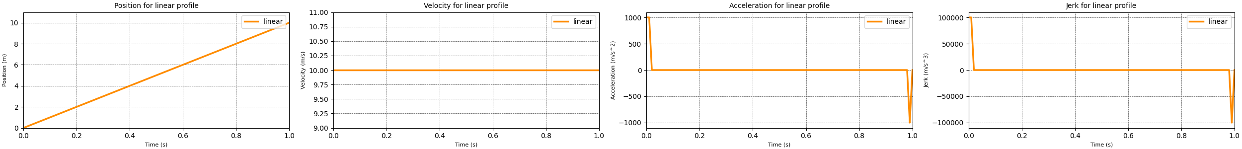
With that you can probably imagine what happens if the velocity has a change from a linearly increasing value to a constant value. The acceleration drops from a positive constant value to zero. And the jerk value displays spikes when the acceleration changes. For the linear motion profile this behaviour is amplified as shown in the plot below. The change in position requires a constant value for velocity which requires significant acceleration and jerk spikes at the start and end of the motion profile.
So in order to move a robot, or robot part, from one location to another in a way that the jerk values stay manageable we need to control the velocity and acceleration across time. This is normally done using a motion profile which describes how the velocity and acceleration change over time in order to arrive at the new state at the desired point in time. Two of the most well known motion profiles are the trapezoidal profile and the s-curve profile.
The trapezoidal motion profile
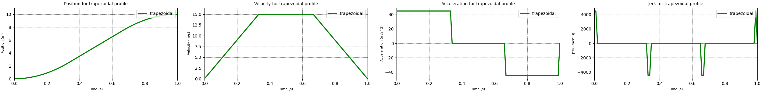
The trapezoidal motion profile consist of three distinct phases. During the first phase a constant positive acceleration is applied. This leads to a linearly increasing velocity until the maximum velocity is achieved. During the second phase no acceleration is applied, keeping the velocity constant. Finally in the third phase a constant negative acceleration is applied, leading to a decreasing velocity until the velocity becomes zero.
The equations for the different phases are as follows
The acceleration, velocity and position in each phase of the trapezoidal motion profile can be described with the standard equations of motion.
Where
t is the amount of time spend in the current phase.n is the current phase
For my calculations I assumed that the acceleration phase and the deceleration phase take the same amount of time, thus they have the same acceleration magnitude but different signs. With this the differences for each phase are:
a(t) = a_{{max}} a(t) = 0 a(t) = -a_{{max}}
My implementation
To simplify my implementation of the trapezoidal motion profile I assumed that the different stages of the profile all take the same amount of time, i.e. one third of the total time. In real life this may not be true because the amounts of time spend in the different stages depend on the maximum reachable acceleration and velocity as well as the minimum and maximum time in which the profile needs to be achieved. Making this assumption simplifies the initial implementation. At a later stage I will come back and implement more realistic profile behaviour.
Additionally my motion profile code assumes that the motion profile is stored for a relative timespan of 1 unit. If I want a different timespan I can just multiply by the desired timespan to get the final result. For this case we can now determine what the maximum velocity is that we need in order to travel the desired distance.
Where
t_{{accelerate}} is the total time during which there is a positive acceleration, which is one third of the total time.t_{{constant}} is the time during which there is a constant velocity, which is also one third of the total time.t_{{decelerate}} is the time during which there is a negative acceleration, which again is one third of the total time.
Simplifying leads to
Using this maximum velocity and the equations for the different phases I implemented a trapezoidal motion profile. The results from running this motion profile are displayed in the plots above. These plots show that the trapezoidal has no large spikes in the acceleration profile when compared to the linear motion profile. additionally the jerk spikes for the trapezoidal motion profile are significantly smaller than the ones generated by the linear motion profile. So we can conclude that the trapezoidal motion profile is a better motion profile than the linear profile. However there are still spikes in the jerk values that would be detrimental for both humans and machinery. So it would be worth finding a better motion profile. That motion profile is the s-curve motion profile discussed in the next section.
The s-curve motion profile
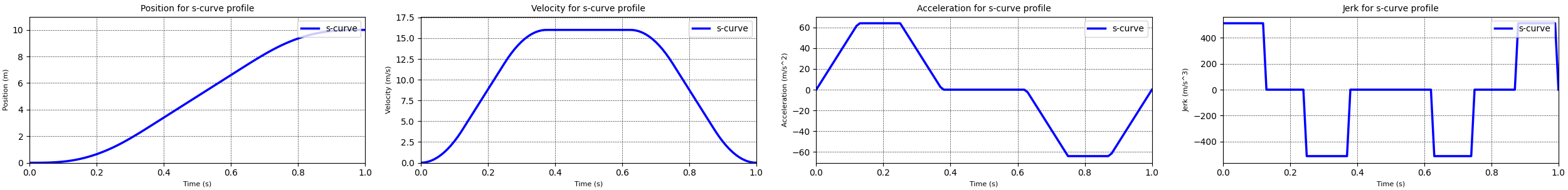
Where the trapezoidal motion profile consisted of three different phases, the s-curve motion profile has seven distinct phases:
- The ramp up phase where a constant positive jerk is applied. Which leads to a linearly increasing acceleration and a velocity ramping up from zero following a second order curve.
- The constant acceleration phase where the jerk is zero. In this phase the velocity is increasing linearly.
- The first ramp down phase where a constant negative jerk is applied. This leads to a linearly decreasing acceleration until zero acceleration is achieved. The velocity is still increasing, following a slowing second order curve to a constant velocity value.
- The constant velocity phase where the jerk and acceleration are both zero.
- The first part of the deceleration phase where a constant negative jerk is applied. Again this leads to a linearly decreasing acceleration, and a velocity decreasing following a second order curve.
- In this phase the acceleration is kept constant and the velocity decreases linearly.
- The final phase where a constant positive jerk is applied with the goal to linearly increase the acceleration until zero acceleration is reached. The velocity will keep decreasing following a second order curve, until it too reaches zero.
As with the trapezoidal motion profile, the acceleration, velocity and position in each phase of the s-curve motion profile can be described with the standard equations of motion. The difference is that the acceleration is a linear function, which introduces a jerk value to the equations.
Where
t is the amount of time spend in the current phase.n is the current phase
As with the trapezoidal motion profile I assumed that the acceleration and deceleration phases span the same amount of time. Again this means the acceleration and deceleration have magnitude but different signs. The differences for each phase are:
j(t) = j_{{max}} j(t) = 0 j(t) = -j_{{max}} j(t) = 0 ,a(t) = 0 j(t) = -j_{{max}} j(t) = 0 j(t) = j_{{max}}
My implementation
To simplify my implementation of the s-curve motion profile I assumed that all stages, except stage 4, all take the same amount of time, i.e. one eight of the total time. I assumed that stage 4 would take one quarter of the time. Like with the trapezoidal profile making this assumption simplifies the initial implementation. At a later stage I will come back and implement more realistic profile behaviour.
Additionally my motion profile code assumes that the motion profile is stored for a relative timespan of 1 unit. If I want a different timespan I can just multiply by the desired timespan to get the final result. For this case we can now determine what the maximum velocity is that we need in order to travel the desired distance.
Using the equations above I implemented a s-curve motion profile. The results from running this motion profile are displayed in the plots above. These plots show that the s-curve removes the spikes in the jerk profile when compared to the trapezoidal motion profile. This indicates that the s-curve motion profile achieves the goal we previously set, to minimize the jerky motion.
For some applications it is important to provide even smoother motions. In this case the motion profiles may need to take into account the values of the fourth, fifth or even sixth order time derivatives of position, snap, crackle and pop. At the moment I have not implemented these higher order motion profiles.
Use in the swerve simulation
Having these motion profiles is great, however by themselves they are of little use. So I added them to my swerve drive simulation to see what the differences were between the different motion profiles.
Before we look at the new results it is worth looking at the simulations using the linear motion profile. I made one for module control and one for body control. In these simulations you can see that with the linear motion profile the jerk spikes are quite large, especially in the case of the module control simulation. The body control approach performs a little better with respect to the maximum levels of jerk, however the values are still far too high.
The simulations for module control and body control using the trapezoidal profile show a significant decrease in the maximum value of the acceleration and jerk values, in some cases by a factor 15. As expected from the previous discussion there are still some spikes, especially for the steering angles. The changes for the module control case are more drastic than for the body control case, probably due to the fact that the values were very high for the combination of the module control with a linear motion profile. Interestingly the acceleration and jerk maximum values are lower for the module control approach than they are for the body control approach. This is most likely due to the fact that in order to keep the drive modules synchronised relatively high steering velocities are required. For instance, the module control approach using the trapezoidal motion profile sees a maximum steering velocity of about 1.8 radians per second. Compare this to the the body control approach with the trapezoidal motion profile which sees a maximum steering velocity of about 3.8 radians per second.
When we look at the simulations using the s-curve motion profile we can see that the maximum acceleration and jerk values actually increase when compared to the trapezoidal motion profile, except for the values of the steering angle jerk when using the module control approach. It seems likely that these increases are due to the fact that the motion is executed over the same time span, but some of the time is used for a more smooth acceleration and deceleration. This means that there is less time available to travel the desired ‘distance’ which then requires higher maximum velocities and maximum accelerations. The s-curve motion profile does smooth out the movement profiles which would lead to a much smoother ride.
What is next
So now that we have a swerve drive simulation that can use both module based control and body based control as well as have different motion profiles, what is next? There are a few improvements that can be made to the simulation code to further made to the simulation and a path of progression.
The first improvement lies in the fact that none of the motion profiles, linear, trapezoidal and s-curve, are aware of motor limits. This means that they will happily command velocity, acceleration and jerk values that a real life motor would not be able to deliver. In order to make the simulation better I would need to add some kind of limits on the maximum reachable values. This would be especially interesting when using body oriented control. Because the high velocities and accelerations are needed to keep the drive modules synchronised. If one of the drive modules is not able to reach the desired velocity or acceleration then the other modules will have to slow down before they reach their limits. To control the drive modules in such a way that all of the modules stay within their motor limits while also keeping them synchronised requires some fancy math. At the moment I'm going through a number of published papers to see what different algorithms are out there.
The second improvement that is on my mind is to implement some form of path tracking, i.e. the ability to follow a given path. This would give the simulation the ability to better show the behaviour of a real life robot. In most cases when a robot is navigating an area the path planning code will constantly be sending movement instructions to ensure that the robot follows the originally planned path. This means that motion profiles need to be updated constantly, which will be a challenge for the simulation code. Additionally having path tracking in the simulation would allow me to experiment with different algorithms for path tracking and trajectory tracking, i.e. the ability to follow a path and prescribe the velocity at every point on the path. And theoretically with a swerve drive it should even be possible for the robot to follow a trajectory while controlling the orientation of the robot body.
Finally the path of progression is to take the controller code that I have written for this simulation and use it with my ROS2 based swerve robot.
In my last two posts I talked about different control methods for a swerve drive robot. One method controls the movement of drive modules directly. The other method controls the movement of the body and derives the desired state for the drive modules from that.
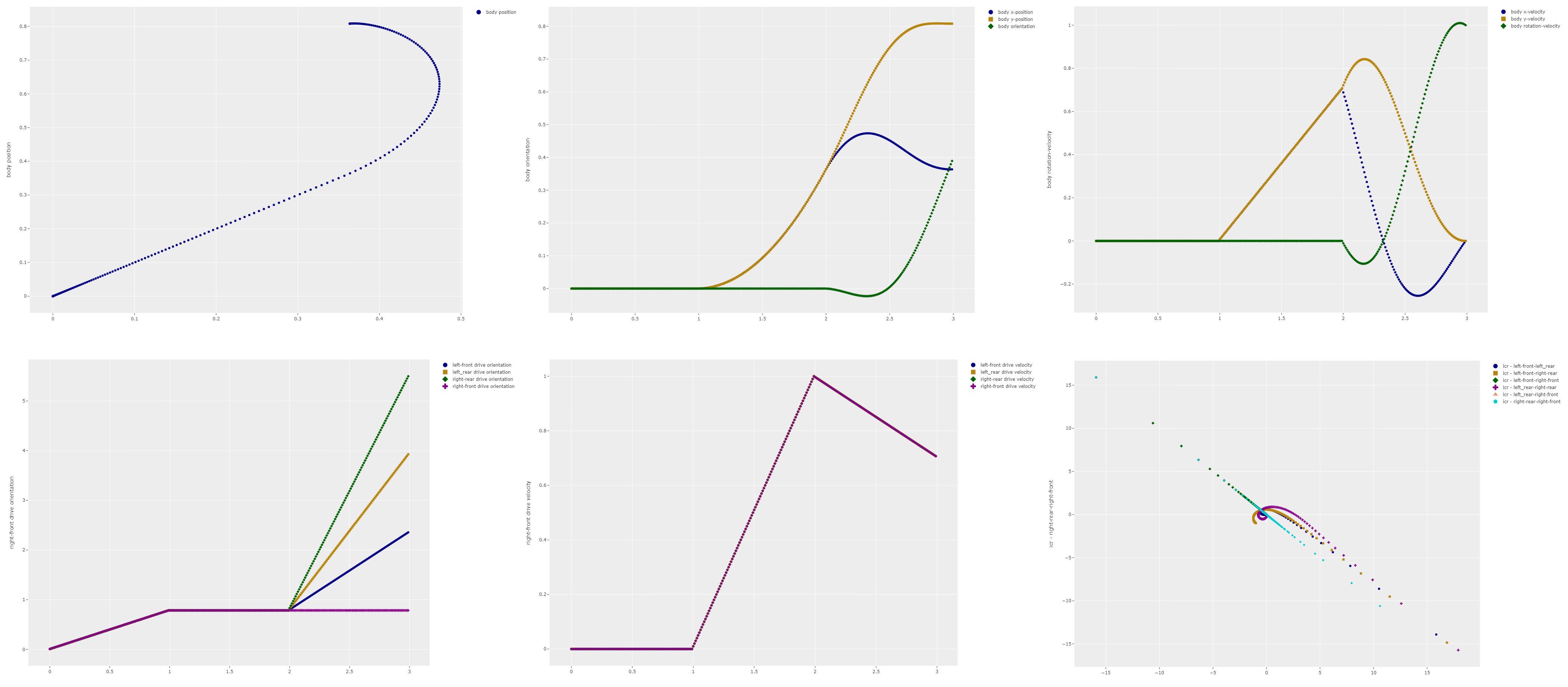
To see the difference between these control methods my simulation code created all kinds of interesting plots like the ones above. However I was still having trouble visualizing what was actually happening, especially in the case of the movement of the Instantaneous Centre of Rotation (ICR), i.e. the rotation point for the robot at a given point in time. The lower left graph shows the paths the ICR for different combinations of drive modules. While it looks pretty it does not make a lot of sense to me.
So to address that issue I updated the simulation code to produce some animations that display the position of the robot and the wheels as well as a number of plots for the state of the robot body and the drive modules. To create the animations I used the FuncAnimation class that is available in matplotlib. The animations can then either be turned into an HTML page with animation controls using the HTMLWriter, or into MP4 video files using the FFMpegWriter. In order to get reasonable performance when using the animation functions in matplotlib it is important to update the plots instead of drawing new ones. This can be done using the set_data function, for instance for updating the position of the robot body. It is good to keep in mind that even with this performance improvement the creation of the animations isn't very fast for our robot simulation because a large number of image frames need to be made. For the 6 second movement in the animation anywhere between 150 and 600 frames need to be created.
The animation above shows how the robot behaves when using the direct module controller. As you can see in the video different pairs of wheels have different rotation points, signified by the red dots. As the movement progresses these rotation points have quite a large range of motion. This indicates that the wheels are not synchronized and most likely some of the wheels are slipping.
I created another animation for the same situation but with the body oriented controller. In this case the rotation points are all in a single location leading me to conclude that all the wheels are synchronized and little to no wheel slip is occurring.
One other interesting thing you can see in the video is that the acceleration and jerk values change very abruptly. In real life this would lead to significant loads on the robot and its drive system. In the simulation this behaviour is due to the fact that linear profile that is being used to transition from one state to another. As mentioned before the next improvement will be to replace this linear interpolation with a control approach that will provide smooth transitions for velocity and accelerations.
Edits
- July 6th 2023: Added a section discussing the use of the matplotlib animation functions.