
Swerve drive - Verification of the kinematics solution
As I explained in an earlier post I have written some code to simulate the movement of a four wheel swerve drive.
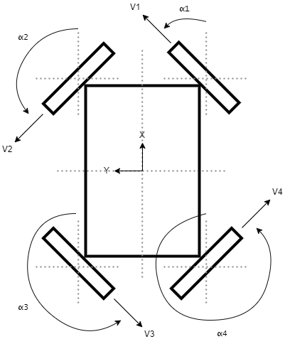
Currently I have only implemented a simple kinematics based approach. This approach is based on the diagram displaying degrees of freedom for the swerve drive as well as the coordinate systems for the different parts. The simple kinematics approach makes a number of assumptions which greatly simplify the problem space.
- The steering axis of a drive module is vertical and passes through the centre of the wheel, i.e. no positional changes occur when the wheel steering angle changes.
- The robot is moving on a flat, horizontal surface, i.e. the contact point between the wheel and the ground is always inline with the steering axis of a drive module.
- The robot has no suspension, i.e. the body doesn't move vertically relative to the contact point between the wheel and the ground.
- There is no wheel slip.
- There is no wheel lift-off, i.e. the wheels of the robot are always in contact with the ground.
- The motors are infinitely powerful and fast, i.e. there are no limits on the motor performance.
With diagram and the given assumptions we can derive the equations for the wheel velocity and the steering angle of each drive module.
v_i = v + W x r_i

alpha_i = acos (v_i_x / |v_i|)
      = asin (v_i_y / |v_i|)
Where
v_i- the wheel velocity of the i-th drive module, i.e. the velocity at which the drive module would move forward if there is no wheel slip. Thexandycomponents of this vector are named asv_i_xandv_i_y.v- the linear velocity of the robot.W- the angular velocity of the robot.r_i- the position vector of the i-th drive module.alpha_i- the steering angle of the i-th drive module relative to the robot coordinate system.
Based on these equations we can determine the forward kinematics, which translates the movement of the drive modules to the movement of the robot body, and the inverse kinematics, which translates the movement of the robot body to the movement of the drive modules. When doing the calculations for a four wheel swerve drive it is important to note that the forward kinematics calculations are overdetermined, i.e. there are more control variables than there are outputs. This means that there are additional control variables that we can play with. One obvious one for a swerve drive is that we can control the orientation of the robot body independent[*] from the direction of movement of the robot. This also means that the forward kinematics calculations are based on the pseudoinverse approach which computes a best fit, a.k.a. least squares, using the drive module wheel velocities and steering angles. In order words the wheel velocities and steering angles are approximations, not exact values.
The transition between states, i.e. from one combination of x-velocity, y-velocity and rotation velocity to another combination, is done by assuming that there is linear control for the drive module variables, i.e. wheel velocity and steering angle. While linear control profiles are not the best control method it does allow later on only changing the profile code to use a more suitable one, for instance a jerk limited profile.
The code I wrote gives me a graphs like the ones presented in my previous post. However before I use this code to test new control algorithms I want to make sure my code is actually producing the correct results. The verification is done by running a bunch of simple simulations for which I am able to predict the behaviour using some simple maths.
To verify that my code is correct I a ran a number of sets of simulations. The first set is used to ensure that both the positive and the negative direction behaviour for the main axis directions. Any differences in behaviour between the positive and the negative direction point to issues in the simulation code. So the simulations that were done for this verification set are:
- Drive the robot in x-direction while facing in the x-direction, one simulation going forward from the origin and one simulation going backwards from the origin.
- Drive the robot in the y-direction while facing in the x-direction, one simulation going left from the origin and one simulation going right from the origin.
- Drive the robot in a rotation only movement, one simulation going clockwise and one simulation going counter-clockwise.
The second simulation set is designed to verify the coordinate calculations related to rotations. The simulations that were done for this verification set are:
- Rotate the robot by 90 degrees and then drive it in the robot x-direction, driving forwards and backwards.
- Rotate the robot by 90 degrees and then drive it in the robot y-direction, driving left and right.
The third set of simulations is designed to verify the behaviour during combined movements. The simulations that were done for this verification set are:
- Drive the robot on the 30 degree diagonals (30 degrees, 60 degrees, 120 degrees, 150 degrees), while facing in the x-direction, one simulation going forwards from the origin and one going backwards from the origin.
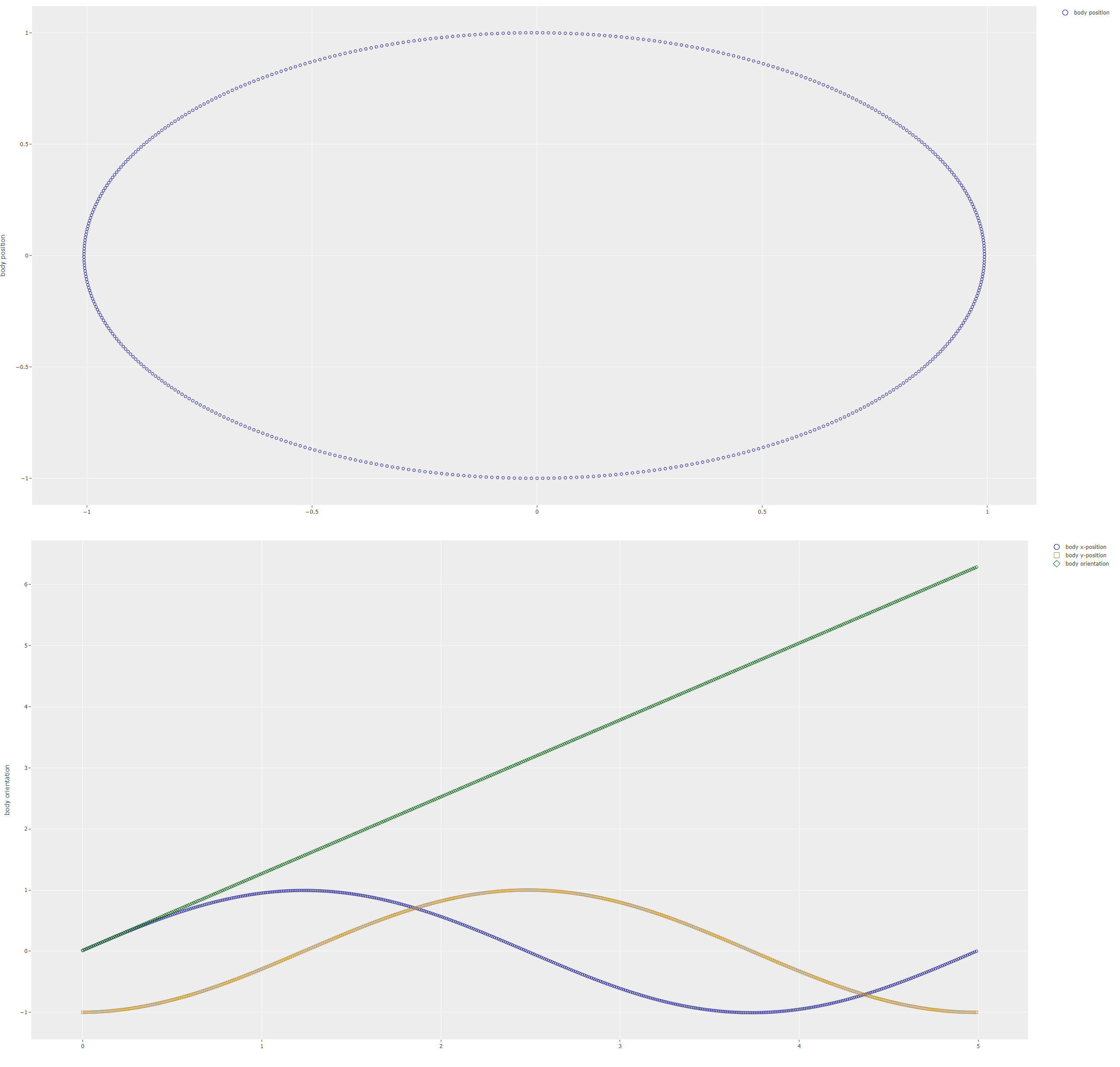
- Drive the robot in a circle around a centre point outside the robot body.
While running the verification sets a number of bugs were found and fixed. At the end of the process all the validations passed indicating that the simulation code is usable.
With all of this done it is now time to do some more complicated simulations both for robot behaviour that is specific to swerve drive systems and for different control algorithms. More on that in the next post.
–
[*] Mostly independent. In reality the motors used in the drive modules will have limits on how fast they can be driven, how much torque they can produce and how fast they can change from one state to the next. This means that there are limitations on movements of the drive modules and thus the robot body. For instance if a drive module has a maximum linear velocity of 1.0 m/s it is not possible to drive the robot diagonally any faster than this velocity, even though we can drive the robot in x-direction at 1.0 m/s and we can drive the robot in y-direction at 1.0 m/s. We just can't do both at the same time.
Edits
- July 4th 2023: Changed the term
control trajectorytocontrol profilebecause the termtrajectoryis generally reserved for path planning situations.