
Swerve drive - Motor limitations
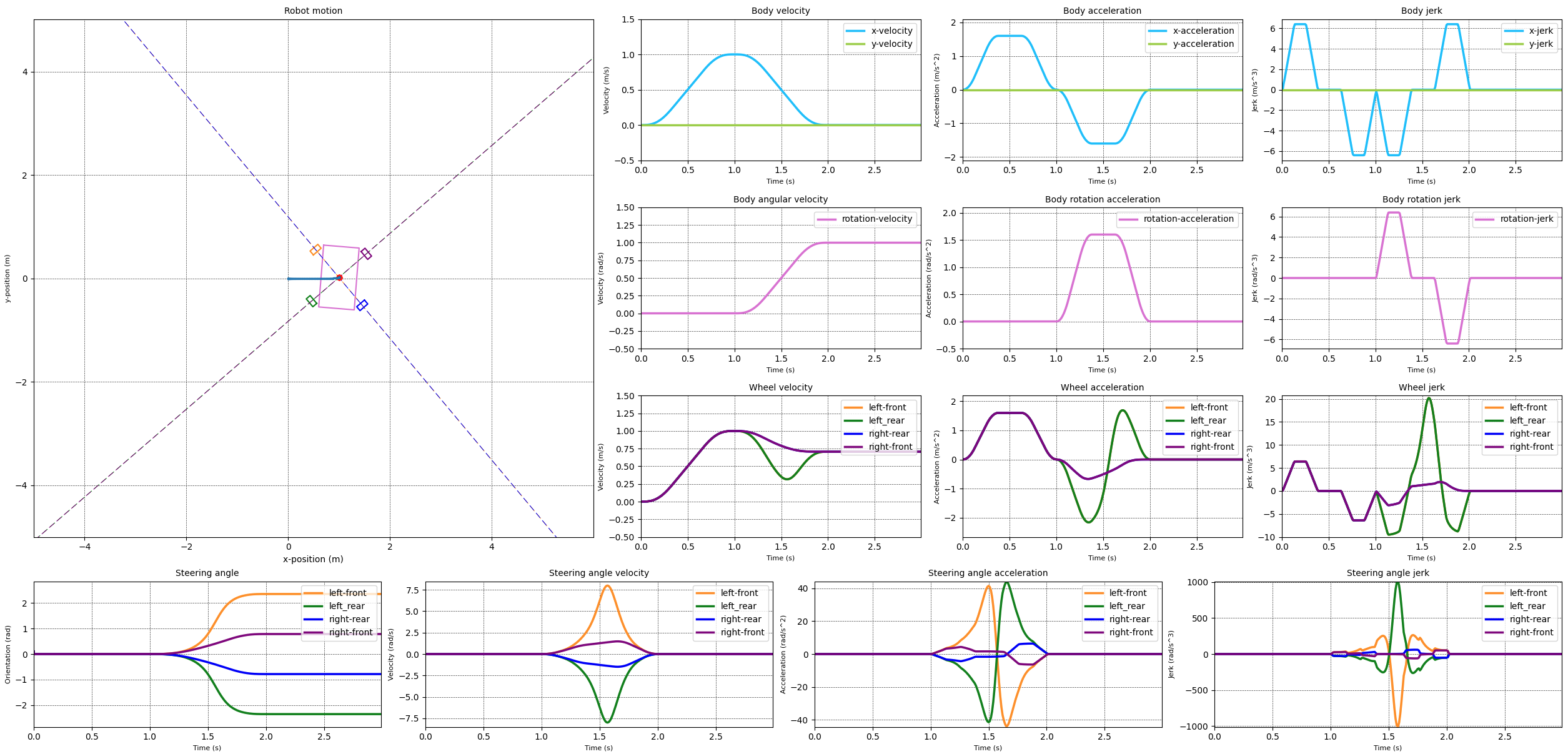
The swerve controller I have implemented so far assumes that the robot is able to follow all the movement commands it has been given. This can lead to extreme velocity and acceleration for the drive and steering motors. The image below shows the result of a simulation where the robot is commanded to move in a straight line followed by a rotate in-place. The simulation used a s-curve motion profile to generate a smooth body movement between different states. The graphs show that the drive velocity and acceleration are smooth and don't reach very high values. It is thus expected that these are well within the capabilities of the drive motors. The steering velocity and acceleration show significant peaks which are likely to tax the steering motors.
In order to ensure that the motors are able to follow the movement commands while keeping the motions of the different drive modules synchronised, we need to take into account the capabilities of the motors.
Now there are many different motor characteristics that we could take into account. For instance:
- The maximum velocity the motor can achieve. This obviously limits how fast the drive module can steer or rotate the wheels.
- The maximum acceleration the motor can achieve. This limits how fast the drive module can change the drive or steering velocity and thus how quickly it can respond to command changes.
- The maximum jerk the motor can achieve. This limits how quickly the motor can achieve the desired acceleration.
- The existence of any motor deadband. This is the region around zero rotation speed where the motor doesn't have enough torque to overcome the static friction of the motor and attached systems. Once enough torque is applied the motor will start running at the rotation speed that it would normally have for that amount of torque. This means that there is a minimum rotation speed that the motor can achieve.
- The behaviour of the motor under load. For instance the motor may not be able to reach the desired rotation speed under load.
- The motor settling time, which is the time it takes the motor to reach the commanded speed.
- The behaviour of the motor when running ‘forwards’ versus when running 'backwards'. For instance the motor may have a different maximum velocity in the ‘forward’ direction than it does in the 'backwards' direction.
At the moment I will only be looking at the maximum motor velocities and the accelerations. These two have a direct effect on the synchronisation between the drive modules. The other characteristics will be dealt at a later stage as they require more information and thought.
In order to limit the steering and drive velocities I've implemented the following process
- Determine the body movement profile that allows the body to achieve the desired movement state in a smooth manner using s-curve motion profiles.
- Divide the body movement profiles into N+1 points, dividing the profile into N sections of equal time. For each of these points calculate the velocity and steering angle for the drive modules. These velocities and steering angles then form the motion profiles for each of the drive modules.
- For each point in time check the steering velocity for each module. Record the maximum velocity of all the profiles. If the maximum velocity is larger than what the motor can deliver then increase or decrease the current timestep in order to limit the steering velocity to the maximum velocity of the motor. Changing the duration of the timestep will change the steering velocities of all the modules. Thus we limit the steering velocities while maintaining synchronisation between the modules.
- Repeat the previous step for the drive velocities.
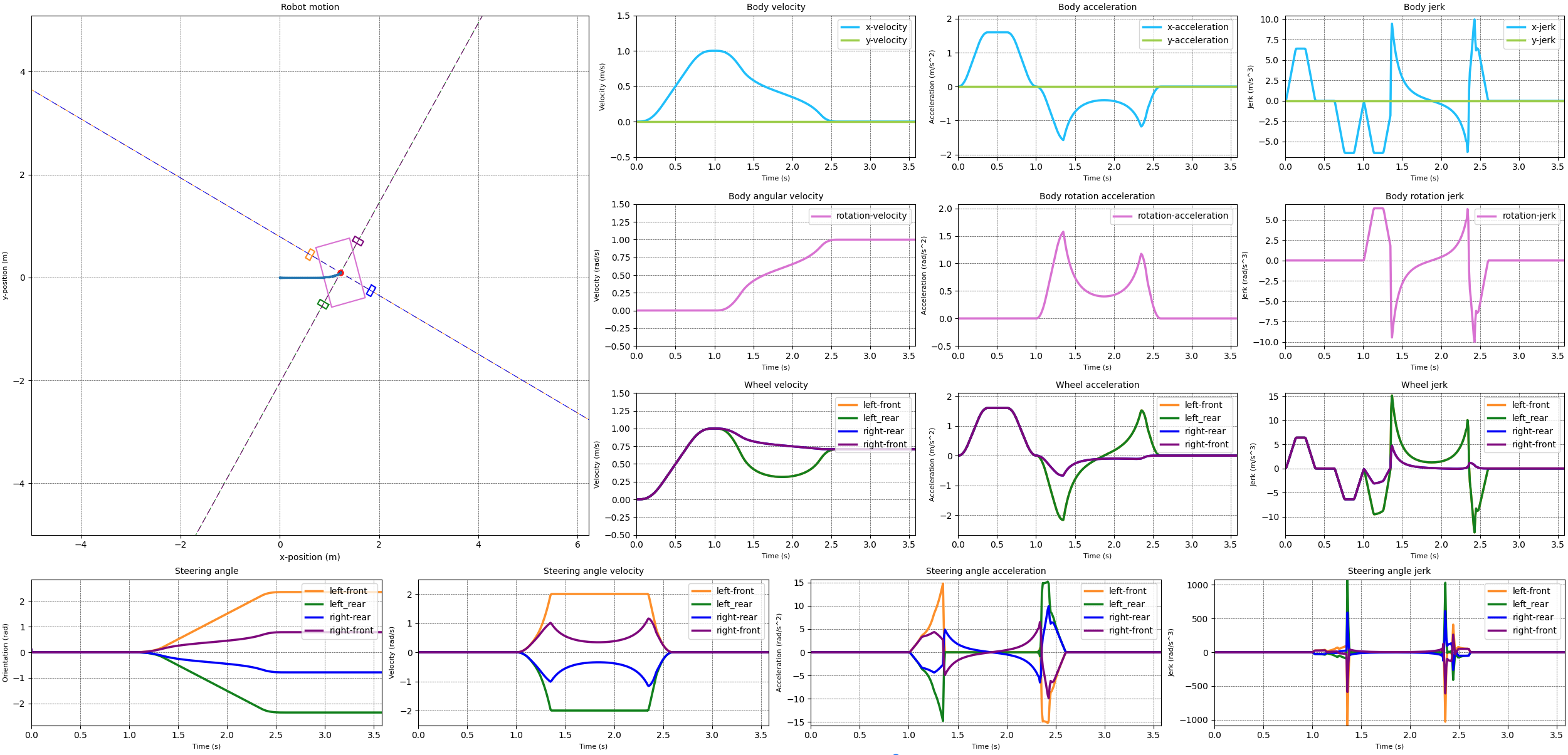
The following video shows the result of the simulation using the new velocity limiter code. The video shows the robot moving in a straight line and then rotating in place. When the rotation starts the steering velocity for the different drive modules increases. As the steering velocity reaches 2 rad/s for the left front and left rear modules the limiter kicks in and maintains that steering velocity. In response the steering velocities of the other wheels reduces in order to keep the drive modules synchronised. The wheel velocities are slightly altered.
With the steering and wheel velocities limited in a reasonable way I attempted to do the same for the steering acceleration. The results of this can be seen in the next images. The first image limits the steering acceleration to 15 rad/s^2. The second image limits the steering acceleration to 10 rad/s^2.
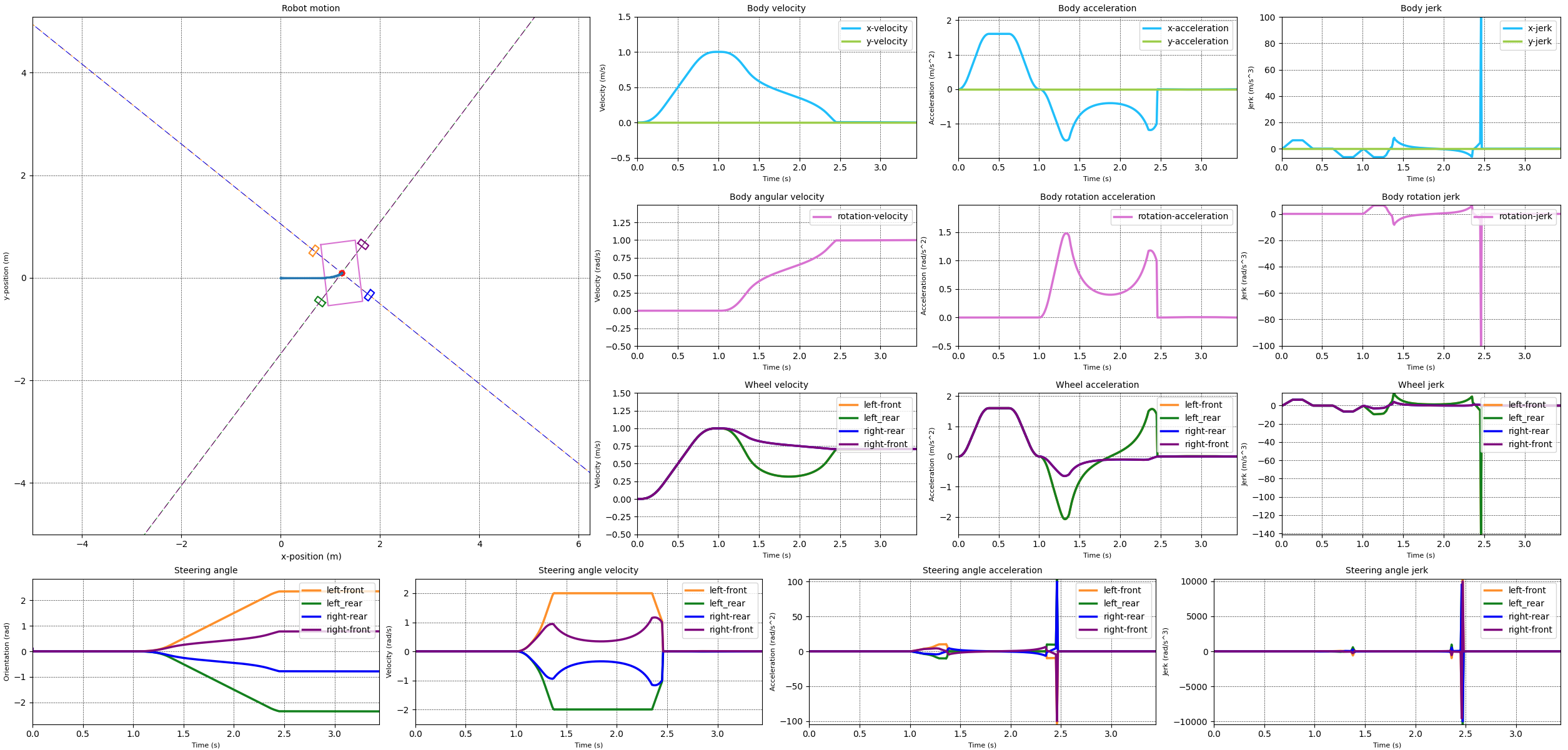
When comparing the two simulation results it becomes clear that something happens if we limit the steering acceleration to 10 rad/s^2. The velocities over all for both cases looks reasonable, except for the 10 rad/s^2 case where the steering velocity snaps to zero at the end of the transition from the straight line to the rotation. This is reflected in a momentary acceleration of over 100 rad/s^2.
The acceleration is calculated based on the difference between the velocity at the current timestep and the velocity at the previous timestep. Additionally the algorithm has to ensure that the steering angle change between the previous and current timestep is controlled so that synchronisation of the drive modules is maintained. Generally to limit the velocity the duration of the timestep is increased. However for the acceleration, especially when decelerating from a positive velocity, there is a limit to how much the timestep can be increased. A larger time step increase decreases the velocity. This then increases the deceleration needed. So this means that you get very large timesteps, or very small timesteps. The current algorithm favours small timesteps.
In either case the problem occurs when slowing down. At the end of the deceleration profile the desired position is achieved, but the velocity and acceleration are not zero. This is not realistic or physically possible. This behaviour is possibly due to the fact that the timesteps are individually calculated. This means that the algorithm doesn't know what the desired end states are and so those are not taken into account.
Additionally if we look at this approach from a higher level we can see that there are two potential areas where improvements can be made in the control model. The first area is related to the fact that the steering velocity and acceleration are computed values, i.e. they are derived from the change in the steering position. This means that there is no direct control over the steering velocity and acceleration. A better algorithm would include these values directly and be able to apply boundary conditions on these values. This could be achieved by extending the current kinematic model with the body accelerations and jerks. The second area is related tot the fact that the module states are derived from the body state. This is necessary to keep the modules synchronised with the body. However this means that the module states are not directly controlled. Which means that it is more difficult to include the module limitations in the control model.
These issues will only become more pronounced if we want to start limiting the maximum jerk values for the steering and drive directions. Limiting the maximum jerk is required to prevent excessive forces on the drive module components.
One possible solution to these issues is to switch to a dynamic model for the control of the robot, i.e. one that is based on the forces and accelerations observed by the robot as it moves. The current model is a kinematic model, i.e. based on the positions and velocities of the different components. Using a dynamic model would allow for the inclusion of the body accelerations and jerks. Additionally the dynamic model would allow for the inclusion of the behaviour of the steering modules more directly and thus lead to a more accurate control model. Finally a dynamic model would also allow for the inclusion of skid and slip conditions as well as three dimensional movement on uneven terrain. The drawback of a dynamic model is that it is more complex and thus requires more effort during implementation and at run time.
At the moment I have not made any decisions on how to progress the swerve controller. It seems logical to implement a dynamic model, however which model should be used and how to implement it requires a bit more research. For the time being I'm planning my next step to be to design and build a single drive module in real life.